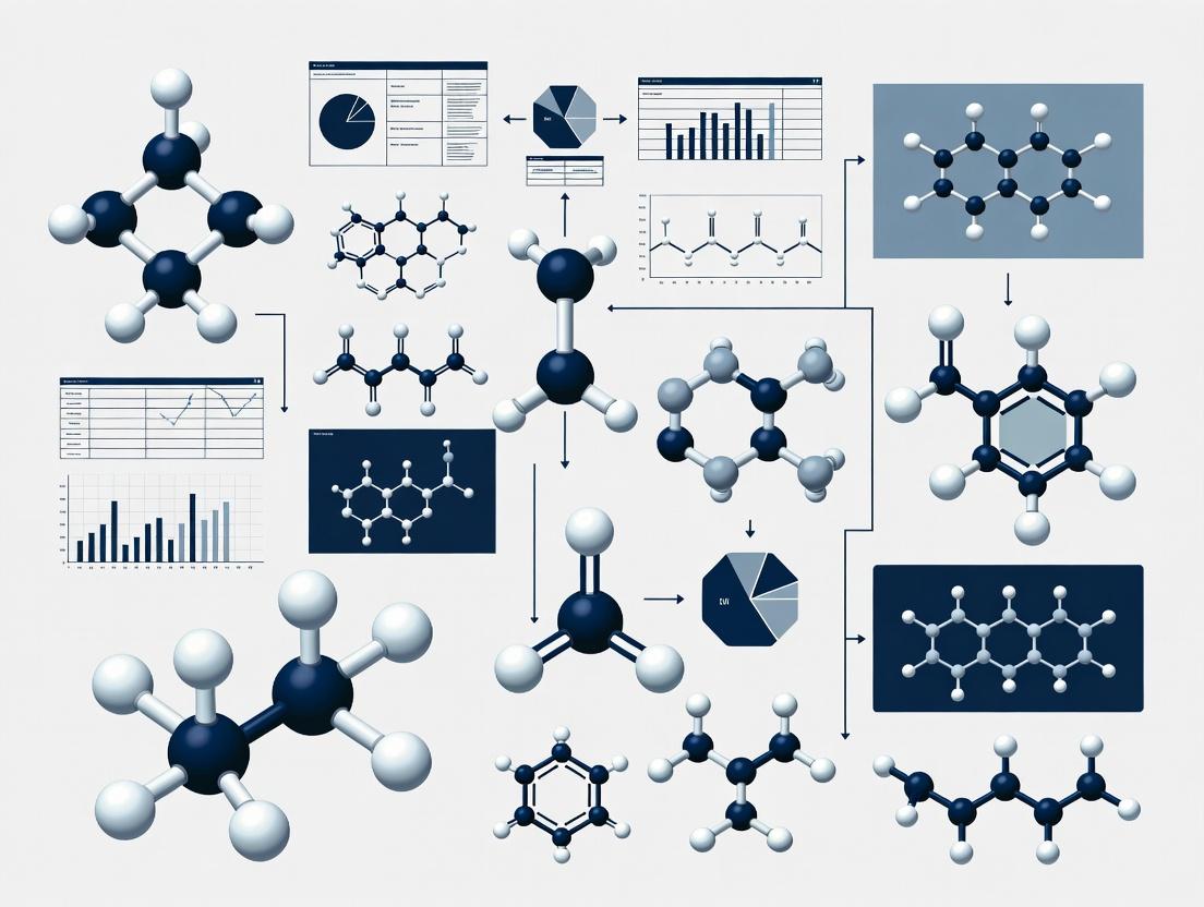
Unlocking Chemical Space: A Guide to 3D Molecular Metrics Analysis for Fragment-Based Drug Discovery Libraries

Abstract

This article provides a comprehensive guide to 3D molecular metrics analysis for fragment libraries, a critical component of modern fragment-based drug discovery (FBDD). Tailored for researchers and drug development professionals, it explores the foundational principles of 3D molecular descriptors and their superiority over traditional 2D metrics in assessing chemical diversity and scaffold complexity. We detail methodologies for calculating and applying key 3D metrics like Principal Moments of Inertia (PMI), Plane of Best Fit (PBF), and 3D Shape Fingerprints to optimize library design. The guide addresses common challenges in property calculation and spatial analysis, offering troubleshooting strategies. Finally, it presents validation frameworks and comparative analyses against 2D methods, highlighting how robust 3D metrics enhance hit identification, lead optimization, and the efficient exploration of bioactive chemical space for novel therapeutics.

Beyond Flatland: Foundational Concepts of 3D Molecular Metrics for Fragment Libraries

1. Introduction and Thesis Context Within the broader thesis on 3D molecular metrics analysis for fragment libraries research, defining and calculating accurate shape descriptors is foundational. Fragment-based drug discovery (FBDD) leverages small, low-molecular-weight compounds, where binding is heavily influenced by efficient 3D shape complementarity to the target. Moving beyond simple 1D/2D descriptors, 3D metrics like Principal Moment of Inertia (PMI), Plane of Best Fit (PBF), and advanced shape descriptors are critical for characterizing library shape diversity, identifying isosteric replacements, and understanding pharmacophore space. This protocol details their calculation and application.

2. Core 3D Molecular Metrics: Definitions and Calculations

2.1 Principal Moments of Inertia (PMI) Ratio PMI analyzes molecular shape by calculating the three principal moments of inertia (I₁ ≤ I₂ ≤ I₃) for a molecule, treated as a collection of points with atomic masses. The normalized ratios NPR1 = I₁/I₃ and NPR2 = I₂/I₃ project molecular shape onto a triangular plot whose corners represent ideal shapes: rod (1,1), disc (0.5, 1), and sphere (0.33, 0.67). Protocol:

• Input: Generate a valid, energy-minimized 3D conformation (e.g., using RDKit, OMEGA, or CORINA).
• Alignment: Align the molecule to its principal axes of inertia.
• Calculation: Compute eigenvalues (I₁, I₂, I₃) of the inertia tensor.
• Normalization: Calculate NPR1 = I₁/I₃ and NPR2 = I₂/I₃.
• Plotting: Plot the point (NPR1, NPR2) on a triangular graph with the defined corner coordinates.

2.2 Plane of Best Fit (PBF) PBF quantifies the planarity of a molecule. It is defined as the mean of the absolute distances (dᵢ) of all heavy atoms from the least-squares plane through the molecular structure, normalized by the radius of gyration (Rg). Lower PBF values indicate higher planarity. Formula: PBF = (Σ|dᵢ| / N) / Rg Protocol:

• Input: Use the same aligned conformation as for PMI.
• Plane Fitting: Perform a least-squares plane fit to the coordinates of all heavy atoms.
• Distance Calculation: For each heavy atom, calculate the perpendicular distance (dᵢ) to the fitted plane.
• Radius of Gyration: Compute Rg = √(Σ mᵢ rᵢ² / Σ mᵢ), where mᵢ is atomic mass and rᵢ is distance from centroid.
• Final Calculation: Apply the PBF formula.

2.3 Advanced Shape Descriptors

• Radius of Gyration (Rg): A measure of molecular compactness.
• Molecular Volume/Surface Area: Often calculated via van der Waals or solvent-accessible surfaces.
• Asphericity (Ω): Describes deviation from spherical symmetry. Ω = ( (I₁ - Ī)² + (I₂ - Ī)² + (I₃ - Ī)² ) / (2·Ī²), where Ī is the average moment.
• Eccentricity: Derived from PMI ratios.
• Shape Fingerprints/Overlays: Quantitative comparison of 3D shapes using methods like Ultra-Fast Shape Recognition (USR) or ROCS (Rapid Overlay of Chemical Structures).

3. Quantitative Data Summary

Table 1: Characteristic Ranges for 3D Shape Metrics in Fragment Libraries

Metric	Ideal Rod-like	Ideal Disc-like	Ideal Sphere-like	Typical Fragment Range
NPR1 (I₁/I₃)	~1.0	~0.5	~0.33	0.4 - 0.9
NPR2 (I₂/I₃)	~1.0	~1.0	~0.67	0.6 - 1.0
PBF	Low (<0.1)	Very Low (<0.05)	Higher (>0.2)	0.05 - 0.25
Asphericity (Ω)	High (>0.5)	Moderate	Low (~0)	0.05 - 0.7
Radius of Gyration (Å)	Higher (function of length)	Moderate	Lower (for given mass)	3.0 - 5.5

4. Application Protocol: Analyzing a Fragment Library

Objective: Profile the 3D shape diversity of a proposed fragment library. Workflow:

• Library Preparation: Curate SMILES strings of the fragment library (MW < 300 Da, heavy atom count < 20).
• 3D Conformer Generation: Use a tool like RDKit's ETKDG method or OMEGA to generate one representative, energy-minimized conformation per fragment.
• Batch Calculation: Script the calculation of PMI/NPR, PBF, Rg, and Asphericity for all conformers (using RDKit, Open3DALIGN, or in-house scripts).
• Data Aggregation & Visualization: Populate a data table and create a PMI triangular plot colored by PBF value.
• Diversity Analysis: Cluster fragments based on their shape descriptor vectors to identify over- and under-represented shape classes.
• Targeted Selection: For a given query pharmacophore, use shape similarity (e.g., USR, ROCS TanimotoCombo) to prioritize fragments for screening.

5. Visual Workflow and Relationships

Title: Workflow for 3D Shape Analysis of Fragments

6. The Scientist's Toolkit: Key Reagents & Software

Table 2: Essential Tools for 3D Molecular Metrics Analysis

Item	Category	Function/Brief Explanation
RDKit	Open-Source Cheminformatics	Python library for conformer generation (ETKDG), PMI/PBF calculation, and basic shape analysis.
Open3DALIGN	Open-Source Software	Standalone tool for calculating 3D descriptors, including PMI and shape-based alignment.
OMEGA	Commercial Software (OpenEye)	High-quality, rule-based conformer ensemble generation for accurate 3D representation.
ROCS	Commercial Software (OpenEye)	Performs rapid 3D shape overlays and calculates shape Tanimoto similarity scores.
Schrödinger Suite	Commercial Software	Integrated platform for ligand preparation, conformational sampling, and shape-based screening.
Python/NumPy/SciPy	Programming Environment	Custom scripting for batch processing, data analysis, and visualization of descriptor data.
KNIME or Pipeline Pilot	Workflow Platform	Enables the construction of automated, reproducible workflows for library profiling.
CCDC (Cambridge Crystallographic)	Database	Source of experimentally determined 3D structures for validation of computed conformers.

Within the broader thesis on 3D molecular metrics analysis for fragment-based drug discovery (FBDD), this application note addresses a critical methodological flaw. The over-reliance on 2D descriptors, such as the Fraction of sp³ Carbons (Fsp³) or 2D Plane of Best Fit (PBF), can misrepresent the intrinsic three-dimensional complexity of fragment-sized molecules. This mischaracterization risks skewing library design towards flat, "fern-like" scaffolds that may exhibit poorer developability and limit vector exploration in binding sites. Accurate 3D assessment is paramount for enriching libraries with genuinely complex, lead-like fragments.

Quantitative Comparison of 2D vs. 3D Complexity Metrics

The table below summarizes key descriptors and their limitations/advantages.

Table 1: Comparison of Molecular Complexity Descriptors

Descriptor	Dimension	Calculation Basis	Pros	Cons for Fragment Assessment
Fsp³	2D	(Number of sp³ hybridized carbons) / (Total carbon count)	Simple, fast to compute. Correlates with solubility.	Misses stereochemistry. A chain of sp³ carbons can be linear, not complex.
2D PBF	2D	RMSD of atoms from a plane fitted to the 2D coordinates.	Fast indicator of "flatness".	Inherently ignores 3D conformation. A macrocycle can score as flat.
Principal Moments of Inertia (PMI)	3D	Normalized ratios of moments of inertia (I₁/I₃, I₂/I₃).	Distinguishes rod-, disc-, and sphere-like shapes in 3D.	Requires a valid 3D conformation. Conformer-dependent.
Eccentricity	3D	Derived from PMI: sqrt(1 - (I₁/I₃)²).	Single value (0=sphere, 1=rod). Good for sorting.	Loses nuanced shape information.
Synthetic Complexity (SCScore)	2D/3D	Machine learning model trained on synthetic reactions.	Predicts synthetic accessibility.	Not a direct measure of 3D shape complexity.
3D PBF	3D	RMSD of atoms from a plane fitted to a 3D conformer.	True measure of deviation from a plane in space.	Requires an ensemble of conformers for robust analysis.

Experimental Protocols

Protocol 1: Generating a Conformer Ensemble for 3D Analysis

Objective: To generate a representative low-energy conformer ensemble for a given fragment molecule, enabling robust 3D metric calculation. Materials: See Scientist's Toolkit. Procedure:

• Input Preparation: Provide the fragment structure as a SMILES string or 2D MOL file.
• Initial 3D Generation: Use the RDKit ETKDG method (v3) to produce an initial 3D coordinate set. This method uses distance geometry and experimental torsion angle preferences.

• Conformer Expansion: Use the MMFF94 or UFF force field to generate multiple conformers. Set a limit (e.g., 50) and an energy window (e.g., 10 kcal/mol).

• Geometry Optimization & Minimization: Optimize each conformer using a selected force field (e.g., MMFF94s) with a convergence threshold.

• Clustering: Cluster conformers by root-mean-square deviation (RMSD) of heavy atoms (e.g., using Butina clustering) to remove redundancies.

• Output: Retain the lowest-energy conformer from each major cluster for subsequent 3D metric analysis.

Protocol 2: Calculating and Comparing 2D PBF vs. 3D PBF

Objective: To demonstrate the discrepancy between 2D and 3D assessments of molecular planarity. Procedure:

• 2D PBF Calculation:
  • Generate the molecule and compute the 2D coordinates.
  • Compute the plane of best fit using the 2D (x,y) coordinates, treating the z-coordinate as 0 for all atoms.
  • Calculate the RMSD of all atoms from this plane.
• 3D PBF Calculation:
  • Use a representative low-energy 3D conformer from Protocol 1.
  • Compute the plane of best fit using the actual 3D (x,y,z) coordinates.
  • Calculate the RMSD of all atoms from this 3D plane.
• Comparison: For a non-planar 3D molecule (e.g., a twisted macrocycle or a spiro compound), the 2D PBF will be near 0 (falsely indicating planarity), while the 3D PBF will have a significant positive value, accurately reflecting its 3D nature.

Mandatory Visualizations

Title: Workflow for 3D Conformer-Based Fragment Analysis

Title: Decision Logic for Assessing True 3D Fragment Complexity

The Scientist's Toolkit: Research Reagent Solutions

Table 2: Essential Tools for 3D Fragment Analysis

Item	Function in Protocol	Example/Note
Cheminformatics Toolkit (RDKit)	Open-source core for molecule manipulation, conformer generation, and descriptor calculation.	Primary software library for Protocols 1 & 2.
Conformer Generation Algorithm (ETKDG)	Stochastic distance geometry method incorporating experimental torsion angles for realistic 3D structures.	Critical first step in Protocol 1.
Molecular Force Field (MMFF94s/UFF)	Used for energy minimization and optimization of generated conformers.	Ensures physically realistic geometries in Protocol 1.
Clustering Algorithm (Butina)	Groups similar conformers by RMSD to reduce redundancy in the ensemble.	Final step in Protocol 1 to select representatives.
3D Structure File Format (SDF)	Standard format for storing multiple conformers and associated properties.	Output format from Protocol 1, input for visualization.
Molecular Visualization Software (PyMOL, ChimeraX)	For visual inspection of 3D conformers and validation of shape/complexity.	Essential for qualitative check of quantitative results.
Scripting Language (Python)	Glue language to orchestrate the entire workflow from SMILES to final metrics.	Enables automation and batch processing of fragment libraries.

The Role of 3D Diversity in Fragment-Based Drug Discovery (FBDD)

Fragment-Based Drug Discovery (FBDD) is a methodology where libraries of low molecular weight compounds (~150-300 Da) are screened to identify weak binders (fragments) to a biological target, which are then evolved into high-affinity leads. Within the broader thesis on 3D molecular metrics analysis for fragment library design, the concept of 3D diversity is paramount. It asserts that fragments should sample a broad range of three-dimensional shapes and spatial arrangements of pharmacophores, beyond traditional 2D descriptor diversity. This enhances the probability of finding novel, high-quality hits against challenging targets, especially those with flat or featureless binding sites.

Quantitative Metrics for Assessing 3D Diversity

A 3D-diverse fragment library is characterized using metrics derived from conformational analysis. The table below summarizes key quantitative descriptors used in research for evaluating 3D shape and property space.

Table 1: Key 3D Molecular Metrics for Fragment Library Analysis

Metric Category	Specific Metric	Description	Target Range for Fragments
Shape & Geometry	Principal Moments of Inertia (PMI)	Normalized ratios describing molecular shape (rod, disk, sphere).	Broad coverage of PMI triangle.
	Plane of Best Fit (PBF)	Measures "flatness" of a molecule.	<20 for 3D, >35 for flat fragments.
Spatial Property	3D-PSA (Topological)	Polar Surface Area calculated on a single low-energy 3D conformer.	Broad distribution, ~0-100 Ų.
	Fraction of sp³ Carbons (Fsp³)	Measures carbon bond saturation. Higher Fsp³ correlates with 3D shape.	>0.35 preferred for 3D diversity.
Conformational	Number of Rotatable Bonds (NRot)	Count of non-terminal single bonds.	Typically 0-4 for fragments.
	Ring Complexity	e.g., Fraction of chiral centers, fraction of stereocomplex rings.	Higher values indicate complexity.

Application Notes: Designing & Screening a 3D-Diverse Fragment Library

Note 1: Library Design & Curation

• Objective: Construct a fragment library (~1500 compounds) maximizing 3D diversity.
• Protocol:
  • Source Compounds: Apply property filters (MW ≤ 300, ClogP ≤ 3, HBD/HBA ≤ 3/3, RotBonds ≤ 4) to a commercial or in-house collection.
  • Generate 3D Conformers: For each molecule, generate a representative low-energy 3D conformer using software (e.g., OMEGA, CORINA).
  • Calculate 3D Descriptors: Compute metrics from Table 1 for each conformer.
  • Diversity Selection: Use a clustering algorithm (e.g., k-means, sphere exclusion) based on a multi-dimensional space defined by PMI ratios, PBF, and Fsp³. Select one representative fragment from each cluster to ensure maximal shape diversity.
  • Assess Coverage: Visualize the final library in a PMI normalized triangle plot to confirm coverage of rod-like, disk-like, and spherical shapes.

Note 2: Biophysical Screening Cascade

• Objective: Identify binders from the 3D-diverse library against Target X.
• Protocol (Typical Cascade):
  • Primary Screen: Use a high-concentration (0.5-2 mM) biochemical assay or a sensitive biophysical method like Surface Plasmon Resonance (SPR) or ligand-observed NMR (e.g., ¹H CPMG).
  • Confirmatory Assays: Subject primary hits to orthogonal methods. e.g., Microscale Thermophoresis (MST) or Isothermal Titration Calorimetry (ITC) to confirm binding and estimate very weak affinities (Kd ~ µM-mM range).
  • Competition Assays: Use X-ray Crystallography or saturation transfer difference (STD) NMR to determine binding mode and site.
  • Hit Validation: Co-crystallography is the gold standard to provide atomic-level insight for fragment elaboration.

Experimental Protocols

Protocol A: Generating a 3D-Conformer and Calculating PMI/PBF

• Input: SMILES string of a fragment.
• Software: OpenEye toolkit (or RDKit).
• Steps:
  • Generate a single, low-energy 3D conformer using the Omega module.
  • Align the conformer to its principal axes of inertia.
  • Calculate the three principal moments (I₁, I₂, I₃).
  • Compute normalized ratios: i₁ = I₁/I₃, i₂ = I₂/I₃, where I₁ ≤ I₂ ≤ I₃.
  • Calculate PBF: Sum of squared distances of heavy atoms from the least-squares plane, divided by the number of heavy atoms.
• Output: Normalized PMI ratios (i₁, i₂) and PBF value.

Protocol B: Ligand-Observed ¹H NMR Screen (Primary)

• Materials: Target protein (>95% pure), deuterated buffer, DMSO-d6, 3D-fragment library in DMSO stock solutions, 384-well plates, NMR spectrometer.
• Procedure:
  • Prepare samples: Target protein (5-20 µM) in NMR buffer. For each fragment, create a sample with protein + fragment (final conc. 0.2-1 mM, 1-5% DMSO) and a matched control with fragment only.
  • Load samples into 96- or 384-well format NMR tubes/plates compatible with an automated sample changer.
  • Acquire 1D ¹H CPMG spectra with water suppression on all samples.
  • Analysis: Compare peak intensities (line broadening) or chemical shift perturbations (CSP) between the protein-fragment sample and the fragment-only control. Significant changes indicate binding.

The Scientist's Toolkit: Research Reagent Solutions

Table 2: Essential Materials for 3D-FBDD

Item / Reagent	Function / Application
Commercial 3D-Fragment Libraries (e.g., Enamine's 3D-Fragment Set, Life Chemicals F3D)	Pre-curated libraries with enhanced Fsp³ and shape diversity, providing a validated starting point.
OMEGA Conformer Generation Software (OpenEye)	Robust, rule-based system for rapidly generating accurate, multi-conformer 3D models for descriptor calculation.
NMR Screening Kits (e.g., DMSO-d6 stock solutions in 96-well plates)	Enables high-throughput, ligand-observed NMR screening with consistent fragment concentrations and minimized preparation error.
Biacore 8K Series SPR System (Cytiva)	High-throughput, label-free system for primary screening and kinetic characterization of weak fragment-protein interactions.
Mosquito Crystal Liquid Handler (SPT Labtech)	Automates nanoliter-scale crystallization setup, crucial for obtaining fragment co-crystal structures for hit validation.
Panoptic Phosphatase Assay Kit (Thermo Fisher)	Example of a functional biochemical assay compatible with high fragment concentrations for primary screening of enzyme targets.

Visualizations

Diagram 1: 3D-FBDD Workflow from Library to Lead

Title: 3D-FBDD Screening and Optimization Pipeline

Diagram 2: 3D Shape Space Analysis via PMI

Title: Mapping Fragment Shapes in Principal Moment of Inertia Space

The systematic analysis of 3D molecular properties—shape, volume, surface area, and electrostatic potential—is foundational to modern fragment-based drug discovery (FBDD). Within the broader thesis of 3D molecular metrics analysis for fragment libraries, these properties serve as primary descriptors for understanding molecular recognition, predicting binding affinity, and enabling structure-based design. This document provides application notes and detailed protocols for the accurate computation and practical application of these metrics in a research setting.

Quantitative Property Benchmarks for Fragment Libraries

The following table summarizes typical value ranges for key 3D properties across standard fragment libraries, providing a reference for researchers evaluating novel compounds.

Table 1: Typical 3D Property Ranges for Fragment-Sized Molecules

3D Property	Calculation Method	Typical Range (Fragment Library)	Significance in Drug Discovery
Molecular Volume	Van der Waals (VDW) volume using a probe radius (e.g., 1.4 Å for water)	100 – 250 ų	Correlates with molecular weight; crucial for assessing ligand efficiency.
Surface Area	Solvent-accessible surface area (SASA) or molecular surface area (MSA)	150 – 350 Ų	Defines interaction interface; polar SASA predicts desolvation penalty.
Shape Descriptors	Principal moments of inertia (PMI) ratio, asphericity, globularity	PMI ratio: 0.0 (rod) to 1.0 (sphere)	Quantifies molecular shapeliness; spherical fragments often show better solubility and promiscuity.
Electrostatic Potential (ESP)	Surface-averaged potential, or localized extrema (min/max)	-50 to +50 kcal/(mol·e)	Predicts polar interaction sites (H-bonds, salt bridges); guides fragment growing/linking.

Application Notes & Experimental Protocols

Protocol: Computation of Shape, Volume, and Surface Area

Objective: To calculate the key steric properties of fragments from a 3D molecular structure. Software: Open-source tools (RDKit, PyMol) or commercial packages (Schrödinger, MOE).

Procedure:

• Input Preparation: Generate a validated 3D conformation for each fragment. Use conformer generation algorithms (e.g., ETKDG in RDKit) and optimize with the MMFF94 or similar force field.
• Volume Calculation:
  • Import the optimized 3D structure.
  • Define atomic radii (e.g., Bondi radii).
  • Compute Van der Waals volume using a grid-based method or analytical approximation (e.g., Gauss-Bonnet theorem).
  • Record the volume in ų.
• Surface Area Calculation:
  • Using the same structure and radii, calculate the Solvent-accessible Surface Area (SASA).
  • Employ a rolling probe sphere (typically 1.4 Å radius for water).
  • Use the Shrake-Rupley (numeric) or Connolly (analytic) algorithm.
  • Output total SASA and, if needed, decompose into polar/non-polar contributions.
• Shape Descriptor Calculation:
  • Calculate the three principal moments of inertia (I₁, I₂, I₃) from the atomic coordinates and masses.
  • Normalize them: I₁ ≤ I₂ ≤ I₃; I₁ + I₂ + I₃ = 1.
  • Compute the PMI ratio: (I₁/I₃) and (I₂/I₃).
  • Plot fragments on a triangular PMI plot (axes: I₁/I₃, I₂/I₃) to visualize shape diversity.

Workflow for Steric Property Calculation

Protocol: Mapping and Analyzing Electrostatic Potential (ESP)

Objective: To compute and visualize the electrostatic potential on the molecular surface to identify pharmacophore features. Software: Quantum mechanics packages (Gaussian, ORCA), or semi-empirical methods (xtb), combined with visualization tools (VMD, PyMol).

Procedure:

• Structure Optimization: Begin with the optimized 3D conformer from Protocol 3.1.
• Electronic Structure Calculation:
  • Perform a single-point energy calculation using a quantum mechanical method.
  • Recommended Level: DFT (e.g., B3LYP/6-31G*) for accuracy, or faster semi-empirical methods (e.g., GFN2-xTB) for library screening.
  • Output the electron density file (e.g., .cube or .wfn format).
• ESP Calculation:
  • Compute the electrostatic potential on a grid surrounding the molecule using the derived electron density and nuclear charges.
  • V(r) = Σ{nuclei A} (ZA / |R_A - r|) - ∫ (ρ(r') / |r' - r|) dr'
• Surface Mapping & Analysis:
  • Map the calculated ESP values onto an isosurface of the electron density (e.g., 0.001 e/bohr³) or the molecular van der Waals surface.
  • Identify regions of negative (red, acceptor) and positive (blue, donor) potential.
  • Quantify by recording the extreme values (Vmin, Vmax) and calculating the surface-averaged potential or electrostatic moments.

Workflow for Electrostatic Potential Analysis

The Scientist's Toolkit: Essential Research Reagents & Solutions

Table 2: Key Resources for 3D Molecular Metrics Analysis

Item / Solution	Supplier / Software	Function in Protocol
RDKit	Open-Source Cheminformatics	Core library for 3D conformer generation, basic property calculation (volume, SASA), and PMI analysis.
PyMol	Schrödinger (Open-Source variant available)	High-quality molecular visualization, surface generation, and presentation of ESP maps.
GFN2-xTB	Grimme Group (Open-Source)	Fast semi-empirical QM method for calculating electron density and ESP for large fragment libraries.
Multiwfn	Tian Lu (Freeware)	Powerful post-analysis of wavefunctions; calculates ESP, maps it to surfaces, and performs quantitative analysis.
Crystallographic Fragment Library (e.g., F2X-Entry, FragLites)	Various (Commercial & Academic)	Provides experimentally validated 3D fragment structures with binding poses for method calibration.
Cambridge Structural Database (CSD)	CCDC	Repository of experimental small-molecule crystal structures for validating computational geometries and intermolecular interactions.
MMFF94 or GAFF Force Field Parameters	Included in MD packages	Used for geometric optimization and energy minimization of fragment conformers prior to property calculation.

Application Notes

Within the context of a thesis focused on the analysis of fragment libraries using 3D molecular metrics, the selection of a computational toolkit is paramount. These libraries, characterized by low molecular weight and complexity, require precise measurement of 3D characteristics—such as shape, electrostatics, and pharmacophores—to assess diversity, complexity, and potential for binding. The following toolkits represent the core software ecosystems employed in this research domain.

RDKit is an open-source cheminformatics platform widely adopted in academia and industry. Its strengths lie in robust 2D/3D molecular manipulation, descriptor calculation (including 3D descriptors like principal moments of inertia and shape-property maps), and seamless integration with machine learning pipelines. For fragment library analysis, its open nature allows for custom metric development and high-throughput screening of 3D shape similarity.

OpenEye Toolkits, from Cadence Molecular Sciences, are commercial, high-performance libraries renowned for their speed and accuracy in 3D molecular design. Their focus on rigorous science is exemplified by the ROCS (Rapid Overlay of Chemical Shapes) software for shape-based virtual screening and the design of diverse, lead-like libraries. Their toolkits provide exceptional tools for calculating 3D molecular metrics critical for evaluating fragment conformational space and shape diversity.

Schrödinger Suite offers a comprehensive, integrated software platform for drug discovery. Its core strengths include advanced physics-based modeling through the Jaguar quantum mechanics (QM) engine and the Glide molecular docking platform. For fragment analysis, its Phase module provides sophisticated pharmacophore perception and screening, allowing researchers to move beyond simple shape to include critical electronic and steric features in library design and analysis.

The quantitative capabilities of these toolkits for key 3D metric calculations relevant to fragment library research are summarized below.

Table 1: Comparison of 3D Metric Capabilities in Key Toolkits

3D Metric / Feature	RDKit	OpenEye Toolkits	Schrödinger Suite
Conformer Generation	ETKDG (v1-v3) algorithm; Fast, stochastic.	Omega: Rule-based, systematic; High accuracy.	LigPrep: Integrated with force field (OPLS4) minimization.
Shape Similarity	Atom pair/feature-matching based methods.	ROCS: Industry standard Gaussian shape overlay; Tanimoto combo score.	Shape screening in Phase; Complementary to pharmacophore.
Pharmacophore Modeling	Basic pharmacophore feature definitions & searching.	OEChem & OEPharmacophore libraries.	Phase: Detailed perception & flexible alignment.
Quantum Mechanics (QM) Descriptors	Limited; via external integrations.	Limited; focused on MMFF94/AM1-BCC.	Jaguar: High-accuracy QM (DFT) for electrostatic potential, orbital properties.
Primary Use Case in Fragment Analysis	High-volume descriptor calc., custom metric development, ML integration.	High-fidelity shape & electrostatics-based diversity & similarity.	High-end, physics-based profiling of fragment binding characteristics.
Licensing Model	Open-source (BSD).	Commercial, toolkit & application licensing.	Commercial, suite-based subscription.

Experimental Protocols

Protocol 2.1: High-Throughput 3D Shape Diversity Analysis of a Fragment Library Using RDKit

Objective: To generate a diversity ranking of a fragment library based on 3D shape descriptors.

Research Reagent Solutions:

• Input Fragment Library (.sdf/.smi): A collection of fragment-sized molecules (MW <300 Da) in a standardized file format.
• RDKit (v2024.x): Open-source cheminformatics toolkit installed via conda (conda install -c conda-forge rdkit).
• Python Scripting Environment: Jupyter Notebook or standard Python IDE with numpy, pandas, and scikit-learn packages.
• Clustering Algorithm: The scikit-learn implementation of the K-Means or Butina clustering algorithm.

Methodology:

• Library Preparation & Conformer Generation:
  • Load the fragment library SMILES/SDF file using rdkit.Chem.SDMolSupplier() or rdkit.Chem.SmilesMolSupplier().
  • For each molecule, generate a minimum of 50 conformers using the rdkit.Chem.rdDistGeom.ETKDGv3() parameters. Optimize each conformer with the MMFF94 force field using rdkit.Chem.rdForceFieldHelpers.MMFFOptimizeMolecule().
  • Select the lowest energy conformer as the representative 3D structure for each fragment.

• 3D Descriptor Calculation:

  • For each representative conformer, calculate a set of 3D molecular descriptors. Key descriptors for shape include:
    • Principal Moments of Inertia (PMI) descriptors (NPR1, NPR2) using custom RDKit scripts or rdkit.Chem.Descriptors3D.
    • Radius of Gyration (rdkit.Chem.Descriptors3D.RadiusOfGyration).
    • Asphericity and Eccentricity descriptors.
  • Compile all descriptors into a pandas DataFrame, with rows as fragments and columns as descriptors. Standardize the data using sklearn.preprocessing.StandardScaler.

• Diversity Analysis & Clustering:

  • Perform Principal Component Analysis (PCA) on the standardized descriptor matrix to reduce dimensionality.
  • Apply the K-Means clustering algorithm (from sklearn.cluster) on the first 3-5 principal components to group fragments by shape similarity.
  • Visualize the results in 2D or 3D scatter plots (PC1 vs. PC2), colored by cluster assignment.
  • Select one representative fragment from each major cluster to form a shape-diverse subset.

RDKit 3D Shape Diversity Analysis Workflow

Protocol 2.2: Pharmacophore-Based Profiling of a Fragment Library Using Schrödinger Phase

Objective: To identify fragments that match a known pharmacophore hypothesis derived from a target protein's active site.

Research Reagent Solutions:

• Target Structure: High-resolution protein crystal structure (PDB format) with a bound ligand or a known active site.
• Fragment Library Prepared in 3D: A library of 3D fragment structures, typically prepared using Schrödinger's LigPrep.
• Schrödinger Suite (2024-1): Installed with licenses for Maestro, Phase, and LigPrep.
• Computational Resources: Adequate CPU/GPU resources for high-throughput pharmacophore screening.

Methodology:

• Pharmacophore Hypothesis Development:
  • Load the target protein structure into Maestro. Analyze the binding site using the "SiteMap" tool to identify key features (hydrophobic regions, H-bond donors/acceptors).
  • Alternatively, derive a pharmacophore hypothesis from a known active ligand using the "Develop Pharmacophore Model" wizard in Phase. Define features (e.g., A: Hydrogen Bond Acceptor, D: Hydrogen Bond Donor, H: Hydrophobic Group, R: Aromatic Ring).

• Fragment Library Preparation:

  • Prepare the fragment library using the LigPrep module. Generate possible ionization states at biological pH (7.0 ± 2.0), retain specified chiralities, and perform energy minimization using the OPLS4 force field. Output a single, low-energy 3D conformer per fragment.

• Pharmacophore Screening:

  • In Phase, set up a "Pharmacophore Screening" job. Load the prepared fragment library and the pharmacophore hypothesis.
  • Configure screening parameters: set the "Maximum omitted features" to 0 or 1 (strict matching), and define distance matching tolerances (e.g., 1.2 Å).
  • Execute the screening. Phase will flexibly align each fragment to the pharmacophore and score the match based on fit and vector alignment.

• Hit Analysis & Validation:

  • Review the results in Maestro. Sort fragments by Phase HypoScore. Visually inspect the alignment of top-scoring fragments within the pharmacophore.
  • Export the list of matching fragments for further validation via molecular docking (e.g., using Glide).

Pharmacophore Screening Workflow with Schrödinger

From Theory to Practice: Methodologies for Calculating and Applying 3D Fragment Metrics

Within the broader thesis on 3D molecular metrics analysis for fragment-based drug discovery (FBDD) libraries, the generation of relevant, biologically accessible 3D conformers is the foundational step. The subsequent computational analysis—encompassing metrics such as 3D shape similarity, molecular complexity descriptors, and vector-based pharmacophore scoring—is wholly dependent on the quality and relevance of the input conformational ensembles. This protocol details a rigorous, step-by-step methodology for generating conformers suitable for high-resolution metric analysis in fragment library design and prioritization.

Key Concepts and Quantitative Benchmarks

The choice of conformer generation method involves trade-offs between computational cost, conformational coverage, and biological relevance. Recent benchmark studies provide critical quantitative guidance.

Table 1: Performance Comparison of Conformer Generation Tools (Representative Data)

Tool / Algorithm	Typical Number of Conformers per Molecule (Max)	Average RMSD to Crystal Structure (Å)	Computational Speed (Molecules/sec)*	Key Principle
OMEGA (OpenEye)	200-500	0.46 - 0.70	1-10	Systematic, knowledge-based torsion sampling with pruning.
Conformator	50-250	0.48 - 0.75	10-50	Knowledge-based, rule-driven torsion library.
ETKDG (RDKit)	50-200	0.65 - 0.90	50-200	Distance geometry with experimental torsion preferences.
CREST (GFN-FF)	Variable (Boltzmann)	~0.3 - 0.5	0.01-0.1	Genetic algorithm using semi-empirical quantum mechanics.
MACROMODEL (Monte Carlo)	Variable	0.40 - 0.80	0.1-1	Monte Carlo / Low-mode sampling with force field scoring.

*Speed is highly hardware and molecule-dependent. Values are approximate for comparison.

Table 2: Impact of Conformer Count on Metric Analysis Accuracy

Conformer Sampling Level	Coverage of Bioactive Pose (% Success)*	3D Shape Similarity (Tanimoto) Error	Required CPU Time (Relative)	Recommended Use Case
Low (10-50)	65-75%	High Variability	1x (Baseline)	High-Throughput Library Filtering
Medium (50-200)	85-92%	Moderate Reliability	5x - 20x	Standard Metric Analysis & Screening
High (200-1000)	95-98%	High Reliability	50x - 200x	Pharmacophore Analysis & QSAR Modeling
Ensemble (QM-based)	>99%	Highest Reliability	1000x+	Benchmarking & Key Lead Optimization

*Based on benchmarking against CSD (Cambridge Structural Database) small molecule crystal structures.

Experimental Protocols

Protocol 3.1: Standardized Generation for Library Profiling (Using RDKit ETKDG)

This protocol is optimized for generating consistent conformers for 500-10,000 fragment-sized molecules (MW < 300 Da) for initial 3D metric calculations.

• Input Preparation: Supply a standardized SMILES list. Curate salts, neutralize charges (or standardize to a specific model), and remove duplicates.
• Parameterization: Use the ETKDGv3 method. Key parameters:
  • numConfs: 50
  • pruneRmsThresh: 0.5 Å (merges very similar conformers)
  • useExpTorsionAnglePrefs: True
  • useBasicKnowledge: True

• Execution Script (Python):

• Output: An SDF or .mol2 file containing all multi-conformer molecules. Embed metadata (e.g., original SMILES, internal ID) for traceability.

Protocol 3.2: High-Fidelity Generation for Pharmacophore Analysis (Using OMEGA)

This protocol is for generating a diverse, energy-aware ensemble for critical fragments undergoing detailed 3D pharmacophore or shape-based alignment.

• Input Preparation: Use curated, charge-standardized molecules in a single-molecule SDF file.
• Parameterization: Key Omega4 (OpenEye) command-line flags:
  • -maxconfs 200: Increases conformational coverage.
  • -ewindow 15.0: Retains conformers within 15 kcal/mol of the global minimum.
  • -rms 0.5: Pruning RMSD threshold.
  • -strict: Uses stricter parameterization for higher quality.
  • -flipper: Considers alternate protomer/tautomer states.

• Execution Command:

• Post-Processing: Filter output using the -sort flag by energy or RMS diversity. Merge results into the master analysis database.

Protocol 3.3: Validation Against Crystallographic Data

Essential for validating the conformer generation protocol's relevance to experimentally observed geometries.

• Data Curation: Download a relevant test set (e.g., CSD Fragment Subset, PDB binders with MW < 250 Da). Isolate the ligand, remove crystal symmetries.
• Alignment: For each crystal structure, generate an in-silico conformer ensemble (using Protocol 3.1 or 3.2).
• RMSD Calculation: For each molecule, calculate the minimum heavy-atom RMSD between any generated conformer and the crystal structure after optimal alignment. Exclude hydrogens.
• Analysis: Calculate the success rate: percentage of molecules where at least one generated conformer has an RMSD < 1.0 Å (or < 0.5 Å for rigid fragments). Results should meet or exceed benchmarks in Table 1.

Visualization of Workflows

Conformer Generation and Analysis Workflow

Trade-offs in Conformer Generation

The Scientist's Toolkit: Research Reagent Solutions

Table 3: Essential Software and Computational Tools for 3D Conformer Analysis

Item / Software	Primary Function in Conformer Analysis	Typical Use Case in Protocol
RDKit (Open-Source)	Core cheminformatics toolkit; implements ETKDG conformer generation.	Protocol 3.1: Standardized library generation and scripting.
OMEGA (OpenEye)	High-performance, knowledge-based conformer generator.	Protocol 3.2: High-fidelity ensemble generation for key fragments.
CREST (Grimme Group)	Quantum-mechanically driven conformer/rotamer sampling.	Generating benchmark Boltzmann-weighted ensembles for validation.
Cambridge Structural Database (CSD)	Repository of experimental small-molecule crystal structures.	Protocol 3.3: Source of ground-truth geometries for validation.
PyMOL / Maestro	3D molecular visualization and analysis.	Visual inspection of conformer ensembles and RMSD alignments.
Conformer Gallery Scripts	Custom Python scripts to generate composite images of conformer ensembles.	Quality control and reporting of generated conformer diversity.
High-Performance Computing (HPC) Cluster	Parallel processing infrastructure.	Running large-scale conformer generation for entire libraries (>10k molecules).
SQL/NoSQL Molecular Database	e.g., MongoDB with RDKit cartridge, PostgreSQL.	Storing, retrieving, and querying multi-conformer molecules and associated metrics.

Calculating Principal Moments of Inertia (PMI) and Visualizing in Triangle Plots

Within the broader thesis on 3D molecular metrics analysis for fragment libraries research, the calculation of Principal Moments of Inertia (PMI) and their visualization in triangular plots is a fundamental technique for quantifying molecular shape. This protocol details the methodologies for computing PMI ratios from 3D molecular structures and translating these values into a visual assessment of shape diversity within a compound collection, a critical parameter in fragment-based drug discovery (FBDD) for exploring chemical space efficiently.

The principal moments of inertia (I1 ≤ I2 ≤ I3) are calculated from the eigenvalues of the inertia tensor of a molecule's 3D structure. These values describe the mass distribution along three orthogonal principal axes. Normalized ratios (I1/I3 and I2/I3) are used to map molecular shape onto a triangular (or 2D) plot, where the vertices represent extreme shapes: rods (I1/I3 ≈ 0, I2/I3 ≈ 0), disks (I1/I3 ≈ 0.5, I2/I3 ≈ 1), and spheres (I1/I3 ≈ 1, I2/I3 ≈ 1). For fragment library analysis, this metric helps ensure coverage of diverse shapes, which is linked to the ability to target diverse protein binding sites.

Experimental Protocol: PMI Calculation and Plotting

Protocol: Calculating PMI from a 3D Molecular Structure

Objective: To compute the normalized PMI ratios for a single, optimized 3D molecular structure.

Materials:

• A single molecule in a confirmed 3D conformation (e.g., SDF, MOL2 format).
• Computational chemistry software (e.g., RDKit, OpenBabel, Schrödinger Maestro).

Procedure:

• Structure Preparation: Ensure the input molecule has valid 3D coordinates. If necessary, generate a 3D conformation using an appropriate method (e.g., ETKDG in RDKit) and perform a geometry optimization using a molecular mechanics force field (e.g., MMFF94).
• Inertia Tensor Construction: Calculate the elements of the inertia tensor I relative to the molecular center of mass. For a system of atoms with masses mᵢ and coordinates (xᵢ, yᵢ, zᵢ) relative to the center of mass: Iₓₓ = Σ mᵢ (yᵢ² + zᵢ²) Iᵧᵧ = Σ mᵢ (xᵢ² + zᵢ²) I₂₂ = Σ mᵢ (xᵢ² + yᵢ²) Iₓᵧ = Iᵧₓ = -Σ mᵢ (xᵢ yᵢ) Iₓ₂ = I₂ₓ = -Σ mᵢ (xᵢ zᵢ) Iᵧ₂ = I₂ᵧ = -Σ mᵢ (yᵢ zᵢ)
• Diagonalization: Diagonalize the symmetric 3x3 inertia tensor I to obtain its eigenvalues (λ₁, λ₂, λ₃). These eigenvalues are the principal moments of inertia: I1 = λ₁, I2 = λ₂, I3 = λ₃. Sort them such that I1 ≤ I2 ≤ I3.
• Normalization: Calculate the two normalized ratios used for plotting:
  • npr1 = I1 / I3
  • npr2 = I2 / I3
• Output: Record the molecule identifier, I1, I2, I3, npr1, and npr2.

Protocol: Generating a PMI Triangle Plot for a Fragment Library

Objective: To visualize the shape distribution of an entire fragment library.

Materials:

• A library of molecules (SDF file).
• A scripting environment with RDKit or similar and matplotlib/seaborn for plotting.

Procedure:

• Batch Processing: Apply Protocol 2.1 to every molecule in the input library file. Handle conformational generation and optimization consistently for all members.
• Data Aggregation: Compile the calculated (npr1, npr2) coordinate pairs for all successful calculations into a single table.
• Triangle Plot Construction: a. Create a 2D scatter plot with npr1 on the x-axis and npr2 on the y-axis. b. Set axis limits from 0 to 1. c. Draw guidelines representing the extreme shapes: * Rod Line: From (0,0) to (0.5, 1). Points near this line have I1 << I2 ≈ I3. * Disk Line: From (0.5, 1) to (1,1). Points near this line have I1 ≈ I2 << I3. * Sphere Corner: The point (1,1). Points cluster here when I1 ≈ I2 ≈ I3. d. Color points by a relevant property (e.g., molecular weight, calculated logP) to add a third dimension of information.
• Analysis: Assess the coverage of the triangular space. A diverse library should populate the entire region, avoiding excessive clustering in any single zone.

Data Presentation

Table 1: PMI Calculations for Example Fragment Molecules

Fragment ID (MW < 300 Da)	I1 (amu*Ų)	I2 (amu*Ų)	I3 (amu*Ų)	npr1 (I1/I3)	npr2 (I2/I3)	Inferred Shape
Frag_001 (Benzene)	88.2	88.2	176.4	0.50	0.50	Disk
Frag_002 (Linear Alkyne)	12.5	1250.7	1250.7	0.01	1.00	Rod
Frag_003 (Adamantane)	456.8	456.8	456.8	1.00	1.00	Sphere
Frag_004 (Bicyclic)	203.4	587.9	721.3	0.28	0.81	Intermediate

Table 2: Shape Classification Based on PMI Ratios

Shape Region	npr1 (I1/I3) Range	npr2 (I2/I3) Range	Typical Structural Features
Rod-like	0.00 – 0.20	0.90 – 1.00	Linear, elongated molecules (e.g., diacetylenes).
Disk-like / Planar	0.40 – 0.60	0.95 – 1.00	Aromatic systems, flat heterocycles (e.g., porphyrin).
Sphere-like	0.90 – 1.00	0.90 – 1.00	Highly symmetric, 3D molecules (e.g., cubane, adamantane).
Intermediate	All other values	All other values	The majority of molecules with complex topology.

Visualizations

Title: PMI Calculation and Visualization Workflow

Title: Interpretation of PMI Triangular Plot

The Scientist's Toolkit: Research Reagent Solutions

Item/Category	Example/Representative Tool	Function in PMI Analysis
3D Conformer Generator	RDKit (ETKDG Method), OMEGA (OpenEye), CONFGEN (Schrödinger)	Generates physically reasonable 3D molecular structures from 1D or 2D representations, which is the essential starting point for inertia tensor calculation.
Molecular Mechanics Engine	MMFF94, UFF, GAFF (as implemented in RDKit, OpenBabel, Amber)	Performs rapid geometry optimization of generated 3D conformers to obtain low-energy, stable structures for accurate PMI calculation.
Computational Chemistry Suite	Schrödinger Maestro, MOE (Molecular Operating Environment), CCDC Software	Provides integrated, GUI-driven workflows for batch calculation of molecular properties, including moments of inertia, often with built-in visualization.
Programming/Chemoinformatics Library	RDKit (Python), ChemAxon JChem, CDK (Chemistry Development Kit)	Enables custom scripting for high-throughput, automated PMI calculation and data processing across entire fragment libraries.
Data Analysis & Visualization Library	Matplotlib, Seaborn, Plotly (Python), R ggplot2	Used to create the triangular scatter plots from calculated PMI ratios, allowing for color-coding and statistical analysis of shape distribution.
Curated Fragment Libraries	F2X-Entry, F2X-Universal (Arctoris), various commercial & in-house libraries	Provide well-characterized, diverse sets of fragment molecules as the primary subject for PMI-based shape diversity analysis in FBDD campaigns.

Assecting Scaffold Complexity with Plane of Best Fit (PBF) and Radius of Gyration

Within the broader thesis on 3D molecular metrics analysis for fragment libraries research, assessing scaffold complexity is paramount. Fragment-Based Drug Discovery (FBDD) relies on small, low-molecular-weight compounds. A key hypothesis is that fragments with greater three-dimensional (3D) character and scaffold complexity are more likely to yield high-quality lead compounds with better physicochemical properties and selectivity profiles. This application note details the concurrent use of two complementary metrics—Plane of Best Fit (PBF) and Radius of Gyration (RG)—to quantitatively assess and classify the 3D complexity of molecular scaffolds, moving beyond traditional flatness measures.

Theoretical Background & Metrics Definition

• Plane of Best Fit (PBF): A metric quantifying the deviation of a molecule's heavy atoms from a best-fit plane. Calculated as the root-mean-square distance (RMSD) of heavy atoms to the plane. Lower PBF values indicate a flatter, more 2D-like molecule; higher values denote greater 3D character.
• Radius of Gyration (RG): A measure of the spatial distribution of a molecule's atomic mass relative to its center of mass. It describes the "spread" or compactness of the molecule. A larger RG suggests a more extended structure, while a smaller RG indicates a more compact, globular shape.
• Synergistic Interpretation: PBF and RG together provide a nuanced view. A molecule can have high 3D character (high PBF) yet be compact (low RG), indicative of a fused, bridged, or caged system. Conversely, a molecule can be flat (low PBF) but extended (high RG), such as a linear polyaromatic system.

Table 1: Benchmark PBF and RG Values for Common Scaffold Types

Scaffold Type	Example Core	Avg. PBF (Å)	Avg. RG (Å)	Complexity Classification
Flat Aromatic	Benzene, Naphthalene	0.05 - 0.15	1.8 - 2.5	Low (2D, Compact)
Fused/Aliphatic	Decalin, Adamantane	0.40 - 0.70	2.5 - 3.5	Medium (3D, Compact)
Sp³-Rich, Extended	Linear Peptide Mimetic	0.60 - 1.20	4.0 - 6.0+	Medium (3D, Extended)
Complex, Saturated	Steroid Core	0.80 - 1.50	3.5 - 4.5	High (3D, Semi-Extended)

Table 2: Analysis of a Hypothetical Fragment Library (n=500)

Metric	Minimum	Maximum	Mean	Std. Dev.	Target Range for "3D Fragments"
PBF (Å)	0.03	1.82	0.45	0.32	PBF > 0.5
RG (Å)	1.65	6.89	3.21	0.87	Context-Dependent

Experimental Protocols

Protocol 1: Computational Calculation of PBF and RG

Objective: To calculate PBF and RG for a set of molecular structures in an automated workflow.

Materials: See Scientist's Toolkit.

Methodology:

• Input Preparation: Prepare an SDF or MOL2 file containing energetically minimized 3D structures of the molecules. Ensure protonation states are correct for the pH of interest (e.g., pH 7.4).
• Calculation Script (Python using RDKit & NumPy):

• Data Output: Export results to a CSV file for subsequent analysis and visualization.

Protocol 2: Visual Classification & Scatter Plot Analysis

Objective: To visualize and classify fragments based on PBF vs. RG scatter plots.

Methodology:

• Using the data from Protocol 1, create a 2D scatter plot with PBF on the x-axis and RG on the y-axis.
• Establish heuristic classification quadrants based on library statistics or predefined thresholds (e.g., PBF median = 0.45 Å, RG median = 3.2 Å).
  • Quadrant I (Top Right): High PBF, High RG. Extended 3D Fragments.
  • Quadrant II (Top Left): Low PBF, High RG. Flat, Extended Fragments (e.g., rods).
  • Quadrant III (Bottom Left): Low PBF, Low RG. Flat, Compact Fragments (traditional aromatic rings).
  • Quadrant IV (Bottom Right): High PBF, Low RG. 3D, Compact Fragments (privileged, saturated cores).
• Select representative hits from each quadrant for further synthesis or screening prioritization.

Mandatory Visualizations

PBF and RG Analysis Workflow for Fragment Libraries

Logical Relationship of Metrics within Thesis

The Scientist's Toolkit

Table 3: Essential Research Reagent Solutions & Materials

Item / Software	Function in Protocol	Key Notes
RDKit (Open-Source)	Core cheminformatics toolkit for reading molecules, handling conformers, and basic geometry calculations.	Essential for Python scripting. Use GetConformer() and atomic coordinate access.
NumPy & SciPy (Python)	Perform efficient numerical linear algebra for PCA (Plane of Best Fit) and distance/mass-weighted calculations.	Required for covariance matrix and eigenvalue decomposition.
3D Structure File (SDF/MOL2)	Input data containing the 3D atomic coordinates of the fragment library.	Structures must be pre-minimized using a force field (e.g., MMFF94).
Conformer Generation Software (e.g., OMEGA, CONFAB)	Generates representative low-energy 3D conformers if starting from 2D structures.	Critical for accurate PBF calculation; use an ensemble approach (average across low-energy conformers).
Jupyter Notebook / Python IDE	Environment for developing, running, and documenting the analysis scripts.	Enables interactive data exploration and visualization.
Data Visualization Library (e.g., Matplotlib, Seaborn)	Creates the essential PBF vs. RG scatter plots for visual classification and analysis.	Allows coloring by additional properties (e.g., molecular weight, logP).

Applying 3D Shape Fingerprints and Pharmacophore Features for Diversity Analysis

This work constitutes a critical experimental chapter of a broader thesis investigating advanced 3D molecular metrics for the analysis of fragment libraries. The core hypothesis posits that combining volumetric shape descriptors with pharmacophoric feature points provides a superior and more chemically meaningful assessment of library diversity than traditional 2D descriptors, directly impacting hit identification and fragment evolution strategies in drug discovery.

Key Concepts and Quantitative Data

3D Shape Fingerprints: Typically encoded as smooth overlap of atomic positions (SOAP) descriptors or spherical harmonic-based vectors. They quantify the volumetric occupancy and electron density distribution of a molecule. Pharmacophore Features: Abstract representations of chemical functionalities (e.g., Hydrogen Bond Donor (HBD), Hydrogen Bond Acceptor (HBA), Aromatic Ring (AR), Positive/Negative Ionizable (PI/NI), Hydrophobic (H)) critical for molecular recognition.

Table 1: Comparison of Diversity Metrics for a Model Fragment Library (n=5000)

Descriptor Type	Metric	Value for Test Library	Interpretation
2D (ECFP4)	Mean Tanimoto Similarity	0.18 ± 0.08	Low 2D similarity suggests good diversity.
3D Shape Only	Mean Shape Similarity (ROC Shape Tanimoto)	0.55 ± 0.12	Higher baseline shape similarity is common in fragments.
Pharmacophore Only	Average Pharmacophore Feature Count	3.2 ± 1.1	Typical for small fragments (MW <250 Da).
Combined 3D/Pharm	Diversity Score (1 - Avg. Combined Sim.)	0.72	Integrated score indicates optimal coverage of shape/feature space.
Coverage	% of Reference 3D Pharmacophore Voxels Sampled	67%	Quantifies coverage of potential binding interactions.

Table 2: Analysis of Top Diverse vs. Clustered Fragments

Cluster Group	Count	Avg. Shape Diversity	Avg. # Unique Pharmacophores	Suggested Utility
High-Diversity Core	150	0.91	5.8	Primary screening subset, scaffold hopping.
Shape-Dense Cluster	220	0.45	2.1	Target class-focused, deep exploration.
Feature-Rich Cluster	180	0.62	6.5	Targeting polar binding sites.

Application Notes & Experimental Protocols

Protocol 1: Generation of 3D Conformers and Feature Assignment

• Input: Curated SMILES strings of fragment library (MW <300, heavy atoms ≤22).
• 3D Generation: Use RDKit's ETKDGv3 method. Generate up to 50 conformers per molecule with an energy window of 10 kcal/mol.
• Minimization: Optimize each conformer with the MMFF94s force field.
• Pharmacophore Feature Assignment: Utilize software like Open3DALIGN or PHASE. Define features with the following rules:
  • HBD: N or O with bound hydrogen.
  • HBA: N or O with lone pair.
  • AR: Centroids of aromatic rings.
  • H: Non-polar carbon chains or ring systems.
• Output: A multi-conformer SD file with annotated feature properties.

Protocol 2: Calculation of 3D Shape and Pharmacophore Fingerprints

• Reference Conformer Selection: For each molecule, select the lowest-energy conformer as the reference for analysis.
• Shape Fingerprint Computation:
  • Align all molecules to a common inertial frame.
  • Using the shape-it tool or ROCS-like method, rasterize each molecule into a 3D grid (default 0.5Å spacing).
  • Compute a Gaussian-smoothed volume density.
  • Encode the shape as a real-valued vector (SOAP descriptor) or a binary fingerprint based on occupied voxels.
• Pharmacophore Fingerprint Computation:
  • For each molecule, map all assigned features onto the same 3D grid.
  • Create a 6-layer 3D bit fingerprint (one layer per feature type: HBD, HBA, AR, PI, NI, H). A bit is set to '1' if a feature of that type is present in the corresponding voxel.
  • Alternatively, generate a triangle-based pharmacophore fingerprint encoding distances between feature pairs.
• Combined Descriptor: Concatenate the normalized shape vector and the pharmacophore bit-string (or fingerprint) into a single unified descriptor per molecule.

Protocol 3: Diversity Analysis and Library Profiling

• Distance Matrix Calculation: Compute the pairwise distance matrix for all library molecules using a combined distance metric: D_combined = α * D_shape + β * D_pharm (typical α=0.6, β=0.4). Use cosine distance for shape vectors and Tanimoto distance for pharmacophore fingerprints.
• Dimensionality Reduction: Apply t-Distributed Stochastic Neighbor Embedding (t-SNE) or Principal Component Analysis (PCA) to the combined descriptor matrix to visualize library coverage in 2D/3D.
• Clustering: Perform hierarchical clustering or k-means clustering on the distance matrix to identify structurally similar groups.
• Diversity Selection: Apply MaxMin or sphere-exclusion algorithms on the combined descriptor space to select a maximally diverse subset.
• Coverage Analysis: Measure the fraction of occupied voxels in a consensus 3D pharmacophore feature map sampled by the selected subset.

Title: 3D Diversity Analysis Workflow

Title: Descriptor Space and Diversity Selection

The Scientist's Toolkit: Essential Research Reagents & Software

Table 3: Key Computational Tools and Resources

Item / Software	Provider / Example	Primary Function in Protocol
Cheminformatics Toolkit	RDKit (Open Source)	Core handling of molecules, SMILES I/O, conformer generation (ETKDG), 2D fingerprinting.
3D Shape Alignment/Calculation	Open3DALIGN, ROCS (OpenEye)	Calculation of 3D shape similarity metrics and alignment of volumes.
Pharmacophore Modeling Suite	PHASE (Schrödinger), MOE	Definition, perception, and fingerprinting of pharmacophore features from 3D structures.
SOAP Descriptor Generator	DScribe, in-house scripts	Generation of smooth overlap of atomic positions (SOAP) vectors for machine learning-ready shape encoding.
Diversity Selection Algorithm	RDKit, scikit-learn	Implementation of MaxMin, sphere exclusion, or clustering for subset selection.
High-Performance Computing (HPC) Cluster	Local or Cloud-based	Essential for processing large fragment libraries (10k+ molecules) through computationally intensive 3D steps.
Curated Fragment Library	Enamine, ChemBridge, in-house	High-quality, synthetically tractable starting points with known physicochemical properties.

Application Notes and Protocols

1. Introduction: Thesis Context Within the broader thesis on 3D molecular metrics analysis for fragment libraries research, this protocol details a practical workflow for curating fragment libraries. The goal is to move beyond traditional 2D descriptors (e.g., molecular weight, LogP) and systematically integrate 3D shape and electrostatic properties to enhance library diversity, target relevance, and hit discovery efficiency in structure-based drug discovery.

2. Key 3D Metrics for Fragment Library Curation The following quantitative metrics, derived from tools like RDKit, Open3DALIGN, and shape-based overlays, form the core of the analysis. These metrics should be calculated for all candidates and summarized for library profiling.

Table 1: Core 3D Molecular Metrics for Fragment Analysis

Metric Category	Specific Metric	Target Range (Ideal Fragment)	Purpose in Curation
Shape & Size	Principal Moments of Inertia (I1, I2, I3)	Varies; used for shape comparison	Quantifies 3D elongation and planarity.
	Normalized Principal Moments Ratio (NPR1, NPR2)	NPR2 > 0.5 (for 3D character)	Identifies fragments with 3D/spherical character vs. flat, 2D structures.
	Radius of Gyration	3.0 - 4.5 Å	Measures compactness and spatial extent.
Electrostatics	Dipole Moment Magnitude	1.0 - 4.0 Debye	Indicates polarity and directionality of charge distribution.
	Molecular Electrostatic Potential (MEP) Surface Variance	Compound-specific; used for clustering	Captures complexity of electrostatic patterns for diversity analysis.
Conformational	Number of Low-Energy Conformers (< 5 kcal/mol)	≥ 5 - 10	Ensures conformational flexibility for binding.
	Ratio of Polar Surface Area to Total Surface Area (P-SA/TSA)	0.2 - 0.5	Balances polarity for solubility and target interactions.

3. Experimental Protocol: A Tiered Curation Workflow

Protocol 3.1: Initial Library Preparation and 3D Conformer Generation

• Objective: Generate a reliable, multi-conformer 3D representation for each fragment molecule.
• Materials: 2D SDF file of candidate fragments; RDKit or Open Babel software; high-performance computing cluster or workstation.
• Procedure:
  • Input: Load the 2D fragment structures (SMILES or 2D SDF).
  • Cleaning: Standardize structures (neutralize, remove duplicates, check valency).
  • 3D Generation: Use the ETKDG (Experimental-Torsion basic Knowledge Distance Geometry) method in RDKit.
  • Conformer Sampling: For each fragment, generate 50 initial conformers using ETKDGv3.
  • Geometry Optimization: Minimize each conformer using the MMFF94s force field (max 500 iterations).
  • Energy Filtering: Retain all unique conformers within a 5 kcal/mol window from the global minimum.
  • Output: A multi-conformer 3D SDF file for downstream analysis.

Protocol 3.2: Calculation of 3D Shape and Electrostatic Metrics

• Objective: Compute the metrics listed in Table 1 for the lowest-energy conformer of each fragment.
• Materials: 3D SDF from Protocol 3.1; RDKit; Python scripts with NumPy; Psi4 or Gaussian for advanced electrostatic calculations (optional).
• Procedure:
  • Shape Metrics: For the lowest-energy conformer, calculate the principal moments of inertia. Compute NPR1 = I1/I3 and NPR2 = I2/I3. Calculate the radius of gyration.
  • Electrostatic Metrics: Compute the dipole moment using RDKit's partial charges (or from the force field). For advanced MEP analysis, generate an isosurface and compute the variance of potentials on that surface using a quantum mechanics package (e.g., Psi4 at the HF/6-31G* level) for a subset.
  • Surface Area Metrics: Calculate Total Surface Area (TSA) and Polar Surface Area (PSA) using a van der Waals radius probe.
  • Data Compilation: Compile all metrics into a structured table (e.g., CSV file).

Protocol 3.3: 3D Diversity Selection and Target-Focused Filtering

• Objective: Select a diverse subset based on 3D metrics and optionally filter for a specific target protein's binding site topology.
• Materials: Metric table from Protocol 3.2; Scikit-learn library; PyMOL or OpenEye tools; reference protein active site shape (e.g., from a co-crystal structure).
• Procedure:
  • Descriptor Space Definition: Use a combination of NPR2, radius of gyration, dipole moment, and P-SA/TSA ratio as a 4D descriptor vector for each fragment.
  • Clustering: Apply the k-means++ clustering algorithm on the standardized descriptor vectors. Determine k based on the elbow method and desired library size.
  • Diverse Selection: From each cluster, select the fragment closest to the cluster centroid as a representative.
  • Target-Focused Filtering (Optional): For a specific target, perform a shape-based alignment (e.g., using OpenEye's ROCS) of the diverse subset against a reference ligand or a negative image of the binding site. Rank fragments by shape Tanimoto combo score and filter the final list.

4. Visualization of Workflows and Relationships

Title: 3D Metrics Fragment Curation Workflow

5. The Scientist's Toolkit: Research Reagent Solutions

Table 2: Essential Tools & Resources for 3D Fragment Curation

Tool/Resource	Category	Function in Workflow
RDKit	Open-Source Cheminformatics	Core platform for 2D/3D conversion (ETKDG), conformational sampling, basic metric calculation (PMI, dipole), and PSA/TSA computation.
Open3DALIGN	Open-Source 3D Informatics	Advanced 3D shape alignment and comparison, useful for validating diversity and target-based shape matching.
Psi4 / Gaussian	Computational Chemistry	Quantum mechanical calculations for high-fidelity electrostatic properties (Dipole, MEP) on a critical subset of fragments.
ROCS (OpenEye)	Commercial Software	Gold standard for rapid shape-based screening and overlays against a target pharmacophore or site.
Scikit-learn	Python Machine Learning Library	Performing PCA, k-means clustering, and other multivariate analyses on the compiled 3D metric data for intelligent subset selection.
CSD (Cambridge Structural Database)	Commercial Database	Source of experimental fragment conformations for validation of computational models and inspiration for novel, stable 3D scaffolds.
High-Performance Computing (HPC) Cluster	Infrastructure	Essential for batch processing of conformer generation and QM calculations across thousands of fragments in a feasible time.

Solving the 3D Puzzle: Troubleshooting and Optimizing Your Fragment Library Analysis

Common Pitfalls in Conformer Generation and Their Impact on Metric Accuracy

Within the broader thesis on 3D molecular metrics analysis for fragment libraries research, the accurate generation of molecular conformers is a foundational step. Errors introduced at this stage propagate, compromising downstream metric calculations such as RMSD, torsion fingerprint deviations, and pharmacophore overlay scores, ultimately misguiding fragment-based drug discovery (FBDD) campaigns.

Key Pitfalls and Quantitative Impact

The following table summarizes common pitfalls, their causes, and their demonstrable impact on key 3D metrics.

Table 1: Common Conformer Generation Pitfalls and Metric Impacts

Pitfall Category	Specific Example	Primary Cause	Typical Impact on Metric (RMSD/Energy)	Impact on Library Analysis
Inadequate Sampling	Missing bioactive rotamer for a key side chain (e.g., tyrosine OH).	Insufficient torsional sampling or overly stringent energy cutoff.	RMSD > 2.0 Å for the aligned core; false negative in shape screening.	Reduced hit identification from shape-based virtual screening.
Incorrect Force Field	Wrong partial charges for tautomeric states (e.g., guanidine group).	Use of a generic, non-parameterized force field for unusual chemistry.	Energy error > 5 kcal/mol; misranking of conformer stability.	Skews population analysis and ensemble-averaged properties.
Neglecting Solvent Effects	Incorrect folding of a flexible, polar chain in vacuum.	Gas-phase optimization without implicit/explicit solvent model.	Conformer population shift >30%; RMSD ~1.5 Å for polar groups.	Misrepresents likely binding mode in aqueous or protein environment.
Over-reliance on Crystallography	Using a single, potentially strained, crystal conformation as the only template.	Lack of ensemble generation from the experimental starting point.	Artificially low conformational diversity; metric accuracy is context-dependent.	Fragment library diversity is underestimated, reducing coverage.
Stereochemical Errors	Unspecified chiral centers or incorrect double-bond geometry.	Faulty SMILES parsing or lack of stereochemistry perception.	Catastrophic failure (RMSD > 5 Å); invalid molecular representation.	Entire conformer sets are invalid, rendering all metrics meaningless.

Experimental Protocols for Validation

Protocol 1: Assessing Conformer Generator Performance for a Fragment Library Objective: To evaluate the ability of a conformer generation algorithm to reproduce known bioactive conformations from a crystallographic fragment library (e.g., CSD or PDB).

• Input Dataset Curation: Obtain a reference set of 50-100 fragment-sized molecules (<20 heavy atoms) with high-resolution (<2.0 Å) crystal structures from protein-ligand complexes.
• Conformer Generation: For each molecule's 1D representation (canonical SMILES), generate an ensemble of 3D conformers (default settings, e.g., 50 conformers) using the tool under evaluation (e.g., OMEGA, ConfGen, RDKit ETKDG).
• Alignment & Metric Calculation: For each molecule, align every generated conformer to its crystal structure using a maximum common substructure (MCS) algorithm. Calculate the Root Mean Square Deviation (RMSD) of heavy atoms.
• Success Criteria Definition: Determine the fraction of molecules for which at least one generated conformer has an RMSD ≤ 1.0 Å (or other relevant threshold) to the bioactive pose. Report the minimum RMSD (RMSD_min) for each molecule.
• Statistical Reporting: Calculate the mean and median RMSD_min across the dataset. Present results in a comparative table.

Protocol 2: Quantifying the Impact of Solvent Model on Metric Accuracy Objective: To measure how the choice of implicit solvent in geometry optimization affects key molecular metrics relevant to fragment docking.

• Conformer Sampling: Generate an initial ensemble of 20 conformers for a set of 20 polar, flexible fragments using a vacuum-based method (e.g., RDKit ETKDG).
• Geometry Optimization: Split each ensemble. Optimize one set using a vacuum force field (e.g., MMFF94 in vacuum). Optimize the parallel set using an implicit solvent model (e.g., GB/SA water with the same force field).
• Metric Computation: For each optimized conformer, calculate:
  • Dipole Moment: Using the partial charges from the force field.
  • Solvent Accessible Surface Area (SASA): Using a standard probe radius.
  • Intramolecular H-bond Network: Count and type.
• Analysis: For each fragment, compute the mean absolute difference (MAD) for each metric between the vacuum- and solvent-optimized ensembles. Correlate the magnitude of the difference with molecular properties like formal charge and H-bond donor count.

Visualization of Workflows and Relationships

Diagram Title: Pitfalls in Conformer Generation Disrupt 3D Metrics Workflow

Diagram Title: Validation Protocol for Conformer Generators

The Scientist's Toolkit: Essential Reagents & Software

Table 2: Key Research Reagent Solutions for Conformer Analysis

Item Name	Type (Software/Database)	Primary Function in Context
Cambridge Structural Database (CSD)	Database	Source of high-quality, experimental small-molecule and fragment crystal structures for validation and training.
Protein Data Bank (PDB)	Database	Source of bioactive fragment conformations from protein-ligand complexes.
OMEGA (OpenEye)	Software	Widely-used, robust conformer generation engine with customizable sampling and energy thresholds.
RDKit ETKDG	Software (Algorithm)	Open-source, knowledge-based method for efficient conformer sampling and generation.
ConfGen (Schrödinger)	Software	Conformer generator integrating systematic search and Monte Carlo methods with force field scoring.
MOE Conformational Search	Software Module	Provides multiple search methods (Stochastic, Systematic, LowModeMD) within a molecular modeling suite.
GFN-FF/GFN2-xTB	Software (Method)	Fast, semi-empirical quantum mechanical methods for reliable geometry optimization of diverse fragments.
Cresset FieldTemplater	Software	Generates conformers based on molecular field points, emphasizing pharmacophore-relevant shapes.
PYMOL/Maestro	Visualization Software	Critical for visual inspection and manual validation of generated conformers vs. reference structures.
Python (SciKit-chem, MDAnalysis)	Programming Environment	Custom scripting for batch metric calculation, statistical analysis, and pipeline automation.

Within the broader thesis on 3D molecular metrics analysis of fragment libraries, a critical challenge is the accurate computational representation and handling of "problematic" fragments. These include highly flexible molecules, tautomers, and charged species. Their inherent variability or state-specific properties can lead to significant discrepancies in calculated molecular metrics (e.g., 3D shape descriptors, electrostatic potentials, interaction energies), thereby corrupting structure-activity relationship analyses and virtual screening outcomes.

Quantitative Impact Analysis

The following table summarizes the typical prevalence and computational impact of problematic fragments in commercial libraries, based on recent literature and internal analyses.

Table 1: Prevalence and Impact of Problematic Fragments in Screening Libraries

Fragment Class	Approx. Prevalence in Standard Libraries (%)	Key Impact on 3D Metrics	Common Remediation Strategy
Highly Flexible Molecules (≥10 rotatable bonds)	15-25%	High variance in shape/volume descriptors; poor convergence in conformer generation.	Multi-conformer ensembles; constrained conformational sampling.
Tautomerizable Species	20-30% (of relevant chemotypes)	Large shifts in polarity, H-bond donor/acceptor patterns, and charge distribution.	Enumeration of dominant tautomers at physiological pH (7.4±2).
Charged Species (at pH 7.4)	10-20%	Dominant influence on electrostatic potential and solvation energy; state-dependent docking poses.	Explicit treatment of formal charges; counterion placement for salts.
Combined Challenges (e.g., flexible & charged)	5-10%	Compounded errors; highest risk of misprioritization.	Integrated protocol (see Section 4).

Detailed Experimental Protocols

Protocol 3.1: Multi-State Conformer Generation and Clustering for Flexible Fragments

Objective: Generate a representative, energy-weighted ensemble of 3D conformations for a flexible fragment.

• Input Preparation: Prepare the fragment's SMILES string in a canonical isomeric form.
• Initial Conformer Generation: Use the ETKDGv3 method (implemented in RDKit) with a high generation limit (e.g., 5000 conformers). Set useRandomCoords=True for molecules with >15 rotatable bonds to improve sampling.
• Geometry Optimization & Filtering: Optimize all generated conformers using the MMFF94s force field. Discard conformers with strained intramolecular clashes (MMFF94s energy > 50 kcal/mol relative to the minimum).
• Clustering: Perform RMSD-based clustering (Butina algorithm) on the heavy atoms of the flexible core. Use a cutoff of 1.0 Å. Retain the lowest-energy conformer from each cluster containing >5% of the total population.
• Output: Save the final ensemble (typically 10-50 conformers) as a multi-model SDF file. Annotate each structure with its relative Boltzmann weight derived from the optimized energy.

Protocol 3.2: Tautomer Enumeration and State Selection at Target pH

Objective: Identify and rank the relevant tautomeric forms of a fragment for biological screening.

• Enumeration: Use a robust tool (e.g., the TautomerEnumerator from RDKit or ChemAxon's Marvin) to generate all possible tautomers for the input structure. Limit generation to prototropic tautomerism (H+ migration).
• pKa Prediction & Protonation State: For each unique tautomer, calculate the macroscopic pKa values for all ionizable sites using a physics-based method (e.g., Epik, ChemAxon pKa Plugin). Apply the Henderson-Hasselbalch equation to predict the major microspecies at the target pH (e.g., 7.4 for physiological targets).
• Ranking: Rank the resulting (tautomer, protonation state) pairs by their estimated population at the target pH. Discard all species with a calculated population < 5%.
• Output: For each major species (>5% population), generate a canonical 3D conformation (using Protocol 3.1 for flexible cores). Store the ensemble with metadata for population and tautomer class.

Protocol 3.3: Charge Model Assignment for Charged Species

Objective: Apply appropriate partial charge models to accurately represent the electrostatic profile of charged fragments.

• Formal Charge Assignment: Assign integer formal charges based on the validated protonation state from Protocol 3.2 or salt dissociation.
• Partial Charge Calculation:
  • For small fragments, use ab initio methods: Optimize geometry at the HF/6-31G* level, then calculate electrostatic potential (ESP) charges (e.g., using the Merz-Singh-Kollman scheme) at the B3LYP/6-31G* level.
  • For high-throughput processing, use a fast, semi-empirical method (e.g., AM1-BCC) which is parameterized to reproduce ab initio ESP charges.
• Counterion Placement (for salts): For fragments supplied as salts (e.g., HCl, Na+), place the counterion using a distance-based heuristic (e.g., place Cl- along the protonated N-H vector at a typical N–Cl distance of 2.8 Å). Perform a brief minimization of the ion pair.
• Output: Generate a final 3D structure file (e.g., MOL2) with the assigned partial charges explicitly stored.

Integrated Workflow for Problematic Fragment Curation

Diagram Title: Integrated Curation Workflow for Problematic Fragments

The Scientist's Toolkit: Essential Research Reagent Solutions

Table 2: Key Software Tools and Libraries for Fragment Handling

Item (Software/Library)	Function	Application in Protocols
RDKit (Open Source)	Cheminformatics toolkit.	Core engine for SMILES parsing, tautomer enumeration (v3.7+), ETKDGv3 conformer generation, and basic clustering.
ChemAxon pKa Plugin	Accurate pKa and major microspecies prediction.	Used in Protocol 3.2 for determining the dominant protonation/tautomeric state at physiological pH.
Open Babel / OEchem	Chemical file format conversion and manipulation.	Handles SDF/MOL2 I/O, charge assignment, and salt stripping in preprocessing steps.
Psi4 / Gaussian	Ab initio quantum chemistry packages.	Provides high-accuracy geometry optimization and ESP charge calculation for charged species (Protocol 3.3).
OpenMM or AMBER Tools	Molecular mechanics/dynamics force fields.	Used for advanced conformational sampling of highly flexible molecules and implicit solvation energy calculations.
KNIME or Python (Pandas)	Data pipelining and analysis.	Framework for scripting the integrated workflow, managing metadata, and analyzing resulting 3D metric distributions.

1. Introduction & Thesis Context Within a broader thesis on 3D molecular metrics analysis for fragment-based drug discovery (FBDD), a central technical challenge is the computational screening of ultra-large libraries (>>1 million compounds). The trade-off between computational speed and the accuracy of molecular property predictions directly impacts the feasibility and quality of virtual screening campaigns. These notes provide protocols and data for optimizing key computational parameters in this context.

2. Key Parameter Benchmarks & Data Performance metrics for common docking/scoring and molecular descriptor calculation tools were evaluated using the DEKOIS 2.0 benchmark library and an in-house fragment library of 500,000 compounds. Hardware: Dual Intel Xeon Gold 6248R CPUs, NVIDIA A100 GPU, 512GB RAM.

Table 1: Docking Tool Performance on a 10,000-Molecule Subset

Tool & Scoring Function	Avg. Time/Ligand (s)	Enrichment Factor (EF1%)	RMSD to Co-crystal (Å)
AutoDock Vina (Default)	21.4	12.7	1.85
QuickVina 2	5.2	10.1	2.34
smina (Vinardo)	18.7	15.3	1.72
GNINA (CNN-Score)	47.8*	14.8	1.80

*GPU-accelerated time.

Table 2: Molecular Descriptor Calculation Speed vs. Complexity

Descriptor Set (Tool: RDKit)	Count per Molecule	Time for 100k Molecules (s)	Correlation w/ LogP (R²)
MACCS Keys (166-bit)	166	45	0.62
Morgan FP (Radius 2, 2048-bit)	2048	210	0.85
RDKit 2D Descriptors	208	520	0.92
3D Conformer Generation (MMFF94)	N/A	8900	N/A

3. Experimental Protocols

Protocol 3.1: Tuned Multi-Stage Docking Funnel Objective: To rapidly filter a 1M+ library to a manageable number of high-confidence hits. Materials: Pre-processed ligand library (SMILES format), prepared protein structure (PDB format), high-performance computing cluster. Workflow:

• Stage 1 - Fast Filtering: Generate 3D conformers using RDKit's ETKDG method with maxConfs=1. Screen using QuickVina 2 with low exhaustiveness (e.g., --exhaustiveness=8). Retain top 50,000 compounds by score.
• Stage 2 - Balanced Docking: Redock retained compounds using smina with the Vinardo scoring function and standard exhaustiveness (--exhaustiveness=24). Cluster poses and retain top 5,000.
• Stage 3 - Refined Scoring: For top poses, re-score using a more accurate, slower method (e.g., GNINA with a combined CNN/affinity model or MM/GBSA). Apply consensus scoring from at least two functions. Output final 500 hits for visual inspection.

Protocol 3.2: Parameter Optimization for 3D Shape/Electrostatic Similarity Objective: Optimize the weighting of 3D metrics for virtual screening. Materials: Known active ligands, decoy set, Open3DALIGN or ROCS software. Method:

• Generate a multi-conformer library for all compounds (max 5 conformers per compound).
• For each query active, perform shape overlay using a similarity metric (e.g., Tanimoto Combo in ROCS). Systematically vary the weight of the color force field (electrostatic, pharmacophoric) from 0.0 (pure shape) to 1.0.
• Calculate the EF1% for each weight parameter. Plot EF1% vs. weight to identify the optimal balance for your target class. Our data on kinase fragments suggests an optimal electrostatic weight of 0.3-0.4.

4. Visualization of Workflows

Title: Multi-Stage Docking Funnel for Large Libraries

Title: Optimization Strategies for Computational Screening

5. The Scientist's Toolkit: Essential Research Reagents & Software Table 3: Key Computational Tools & Resources

Item	Function & Rationale
RDKit	Open-source cheminformatics toolkit for molecule standardization, descriptor calculation, and basic conformer generation. Essential for pre-processing.
AutoDock Vina/smina	Robust, widely-used docking engines. smina offers customized scoring functions (like Vinardo) shown to improve accuracy for fragments.
GNINA	Deep learning-based docking/scoring. Uses convolutional neural networks (CNNs) for improved pose prediction and scoring, leveraging GPU acceleration.
ROCS (OpenEye)	Rapid overlay of chemical structures based on 3D shape and "color" fields (pharmacophores). Industry standard for fast 3D similarity screening.
DEKOIS/Benchmark Sets	Public databases of decoys and active ligands for validating docking protocols and calculating enrichment metrics.
High-Throughput Compute Cluster	CPU clusters enable parallel docking of millions of compounds. GPU nodes significantly accelerate ML-based scoring (e.g., GNINA).
Consensus Scoring Scripts	Custom scripts (Python/bash) to aggregate and rank results from multiple scoring functions, reducing false positives.

This application note is situated within a broader thesis on the analysis of 3D molecular metrics for the design and curation of fragment-based drug discovery (FBDD) libraries. The primary challenge is navigating the trade-off between maximizing three-dimensional (3D) diversity—to explore novel chemical space and target unique protein epitopes—and adhering to critical drug-like property filters. These filters include the exclusion of Pan-Assay Interference Compounds (PAINS), the assurance of adequate aqueous solubility for biochemical testing, and the maintenance of synthetic accessibility (SA) for future hit-to-lead optimization. This document provides detailed protocols and analytical frameworks for achieving this balance.

Table 1: Key Property Ranges for High-Quality 3D-Enriched Fragment Libraries

Property	Optimal Range for Fragments	Rationale & Measurement Method
Molecular Weight	150 - 300 Da	Keeps compounds within "fragment space" for efficient exploration.
Heavy Atom Count	10 - 20	Correlates with MW; ensures low complexity.
3D Descriptors	PMI ≥ 0.4; NPR ≥ 2.0	Plane of Best Fit (PBF) ≤ 0.3. Ensures non-flat, shapely structures. Principal Moment of Inertia (PMI) ratio and Normalized Principal Moments Ratios (NPR) quantify deviation from linearity/sphericity.
Calculated LogP (cLogP)	≤ 3.0	Maintains solubility and reduces promiscuity risk.
Rotatable Bonds	≤ 3	Limits flexibility, favoring well-defined binding poses.
Hydrogen Bond Donors	≤ 3	Improves solubility and cell permeability.
Hydrogen Bond Acceptors	≤ 6	Improves solubility and cell permeability.
Aqueous Solubility (logS)	> -4.0 (≥ ~100 µM)	Essential for biochemical assay concentrations (often 0.2-1 mM).
Synthetic Accessibility Score	≤ 4.5 (on 1-10 scale, 1=easy)	Ensures feasible chemistry for analog synthesis.
PAINS Alerts	0	Must exclude all substructures known to cause assay interference.

Table 2: Impact of Property Filters on Virtual Library Curation

Initial Library Size	Post-3D Filter (PMI/NPR)	Post-Drug-like Filter (RO5-like)	Post-PAINS Filter	Post-Solubility/SA Filter	Final Yield
500,000 compounds	~40% (200,000)	~60% of 3D set (120,000)	~95% of previous (114,000)	~50% of previous (57,000)	~11.4%

Core Protocols

Protocol 1: Computational Assessment of 3D Shape Diversity

Objective: To identify and select fragments with high three-dimensional character from a flat compound collection.

Materials:

• Compound library in SMILES or SDF format.
• Computational Chemistry Software: e.g., OpenEye Toolkit, RDKit, Schrödinger Suite.
• High-Performance Computing (HPC) cluster or cloud instance.

Procedure:

• 3D Conformer Generation: For each input SMILES, generate an ensemble of low-energy conformers (e.g., 10-20) using a method like MMFF94s or ETKDG in RDKit. Ensure thorough sampling.
• Descriptor Calculation: For the lowest energy conformer of each molecule, calculate the following:
  • Principal Moments of Inertia (I₁ < I₂ < I₃): Compute from the 3D coordinates.
  • PMI Ratio: Calculate NPR1 = I₁/I₃ and NPR2 = I₂/I₃.
  • Plane of Best Fit (PBF): Fit a plane through all heavy atoms and calculate the sum of squared distances; normalize by the radius of gyration.
• Selection Criteria: Apply filters: NPR2 > 2.0 and PBF < 0.3. This selects molecules that are neither rod-like nor spherical, but disc-like or three-dimensional.
• Diversity Analysis: Cluster the selected 3D fragments using shape-based fingerprints (e.g., USR, SHAP) to ensure broad coverage of shape space.

Data Analysis: Visualize the NPR1 vs. NPR2 scatter plot to map the shape distribution of your library against known flat (e.g., benzene) and 3D (e.g., spirocyclic) reference compounds.

Protocol 2: Integrated PAINS, Solubility, and SA Filtering Workflow

Objective: To concurrently remove compounds with undesirable interference potential, poor solubility, and low synthetic feasibility.

Materials:

• List of 3D-enriched fragments (SMILES format).
• PAINS Filtering Tool: RDKit with PAINS SMARTS patterns, or standalone filters.
• Solubility Prediction Tool: AQUAFAC, ESOL, or ADMET predictor.
• SA Prediction Tool: RAscore, SCScore, or SYBA implemented in RDKit.
• Scripting Environment: Python with Pandas for data aggregation.

Procedure:

• PAINS Filtering:
  • Load the RDKit PAINS SMARTS patterns.
  • For each molecule, check for any substructure matches.
  • Immediately discard any molecule triggering a PAINS alert. Log the alert type.
• Solubility Prediction:
  • For the PAINS-free set, calculate predicted aqueous solubility (logS) using the ESOL model: logS = 0.16 - 0.63*cLogP - 0.0062*MW + 0.066*RB - 0.74*AP. Where AP is aromatic proportion.
  • Apply filter: Predicted logS > -4.0.
• Synthetic Accessibility (SA) Scoring:
  • Calculate an SA score for each soluble compound. Using SCScore (1-5 scale, 5=hard), filter for SCScore < 3.5. Alternatively, use SYBA (higher score = more accessible) and filter for SYBA score > 0.
• Consensus Ranking: Create a composite score for final prioritization: Composite Score = (Normalized SA Score) - (Normalized cLogP) + (Normalized 3D Metric). Rank compounds accordingly.

Data Analysis: Generate a parallel coordinates plot showing the distribution of key properties (cLogP, logS, SA Score, PMI) for the final library to confirm balanced profile.

Visualization of Workflows

Diagram 1: Integrated Library Curation & Screening Workflow

Diagram 2: 3D Shape Analysis & Property Correlation

The Scientist's Toolkit: Research Reagent Solutions

Table 3: Essential Tools for 3D Fragment Library Design & Analysis

Tool / Resource	Function	Example / Vendor
3D Conformer Generator	Produces accurate, low-energy 3D molecular models for shape analysis.	RDKit (ETKDG), OpenEye OMEGA, CONFAB.
Shape Descriptor Calculator	Computes quantitative metrics (PMI, PBF, NPR) to classify molecular shape.	In-house Python scripts using RDKit, Schrödinger's shape_screen.
PAINS Filter	Identifies and flags substructures with known assay interference behavior.	RDKit PAINS SMARTS, ZINC PAINS filter, FAF-Drugs4.
Solubility Predictor	Estimates intrinsic aqueous solubility (logS) from chemical structure.	AQSol, ESOL (RDKit), SwissADME web tool.
Synthetic Accessibility Scorer	Predicts the ease of synthesizing a compound, guiding library feasibility.	RAscore, SCScore, SYBA (all available via RDKit).
High-Throughput Visualization	Enables rapid visual inspection of hits and shape clusters.	SeeSAR (BioSolveIT), PyMOL, Maestro.
Fragment Screening Library	Commercially available, pre-curated libraries with claimed 3D character.	Enamine's 3D Fragment Set, Key Organics Fragments, Life Chemicals F3D.

Application Notes

This document details a systematic approach to diagnose and rectify insufficient three-dimensional (3D) shape diversity within a fragment library for drug discovery. In the context of advancing 3D molecular metrics analysis, the efficient exploration of chemical space is paramount. A library biased toward flat, 2D-like molecules can severely limit the identification of hits against challenging targets with complex, globular binding sites. The following protocol outlines the diagnostic metrics, corrective strategies, and validation steps necessary to ensure a library is enriched for 3D character.

Part 1: Diagnostic Analysis of 3D Shape Diversity

Objective: Quantitatively assess the current library's shape profile using established 3D molecular descriptors.

Key Metrics and Data Presentation:

• Principal Moments of Inertia (PMI) Ratio: Normalized ratios (I1/I3 and I2/I3) classify molecules on a triangular plot from rod-like to disc-like to spherical.
• Plane of Best Fit (PBF): Measures the deviation of atoms from a plane; lower values indicate a flatter molecule.
• Fraction of sp3-Hybridized Carbons (Fsp3): Fsp3 = (Number of sp3 carbons) / (Total carbon count). Higher values often correlate with increased stereochemical complexity and 3D shape.
• Number of Stereocenters: A direct measure of chiral complexity.
• Synthetic Accessibility Score (SAscore): Predicts the ease of synthesis, crucial for evaluating downstream feasibility.

Table 1: Diagnostic 3D Descriptor Analysis for an Example Library (n=1000 fragments)

3D Descriptor	Target Range (Ideal)	Library Average (Pre-Correction)	Interpretation & Risk
Fsp3	>0.36	0.22	High prevalence of flat, aromatic systems. Risk: Poor coverage of protein surface features.
PBF (Å)	<0.20 indicates flatness	0.18	Confirms a bias towards planar molecular architectures.
Molecules in "Spherical" PMI Region	>25%	12%	Severe under-representation of globular, 3D shapes.
Avg. Number of Stereocenters	≥1	0.4	Low chiral content limits shape complexity.
SAscore (1=Easy, 10=Hard)	<4.5	3.8	Current library is synthetically tractable.

Protocol 1.1: Calculating 3D Shape Descriptors

• Input Preparation: Generate a standardized SMILES list of the library. Use a tool like RDKit (Chem.rdmolfiles.MolFromSmiles) to parse molecules.
• 3D Conformation Generation: For each molecule, generate an ensemble of low-energy 3D conformers using ETKDG (Experimental-Torsion basic Knowledge Distance Geometry) algorithm as implemented in RDKit. Retain the lowest energy conformer for analysis.
• Descriptor Calculation:
  • Fsp3: Use RDKit's Descriptors.rdMolDescriptors.CalcFractionCSP3.
  • PMI/NPR: Calculate principal moments of inertia (rdMolDescriptors.CalcPMI1, etc.), normalize, and compute normalized principal moment ratios (NPRs).
  • PBF: For the lowest energy conformer, compute the sum of squared distances of each heavy atom to the least-squares plane. Scripts are available in open-source repositories (e.g., GitHub - rdkit/rdkit).
  • Stereocenters: Use RDKit's Chem.FindMolChiralCenters.
• Visualization: Create a PMI triangular scatter plot (rod-disc-sphere) and histograms for Fsp3 and PBF to visually assess distribution.

Part 2: Corrective Enrichment Protocol

Objective: Systematically select or acquire fragments to shift the library's 3D descriptor profile toward the target ranges.

Strategy: Focus on fragments with high Fsp3, cyclic systems (saturated/heterocycles), and defined stereochemistry, while maintaining drug-like properties (MW <300, cLogP <3, HBD/HBA counts).

Table 2: Research Reagent Solutions for Library Correction

Reagent / Resource	Function in Protocol
RDKit (Open-Source)	Core cheminformatics toolkit for descriptor calculation, conformer generation, and filtering.
ZINC20 / eMolecules Database	Commercial & public compound databases for sourcing purchasable, 3D-enriched fragments.
Enamine REAL Space	Source of synthetically accessible, bespoke fragments with high 3D complexity.
MOE (Molecular Operating Environment)	Alternative commercial software for comprehensive conformational analysis and descriptor calculation.
KNIME Analytics Platform	Workflow automation to integrate data retrieval, descriptor calculation, and multi-parameter filtering.

Protocol 2.1: Multi-Parameter Filtering for 3D Enrichment

• Source a Candidate Pool: Extract fragments from 3D-enriched subsets of commercial databases (e.g., "3D-Fragment" collection from ZINC20) or from lists of saturated/spring heterocycles.
• Apply Property Filters: Filter candidates by: Molecular Weight (MW ≤ 250), Calculated Log P (cLogP ≤ 3), Hydrogen Bond Donors (HBD ≤ 3), Hydrogen Bond Acceptors (HBA ≤ 3).
• Apply 3D Descriptor Filters: Apply sequential filters:
  • Step 1: Fsp3 ≥ 0.36.
  • Step 2: PBF ≥ 0.25 (to exclude flat molecules).
  • Step 3: Ensure presence in the "spherical" or intermediate region of PMI plot (NPR2 > 0.5).
• Assess Synthetic Accessibility: Filter out candidates with SAscore > 5 to maintain future synthetic tractability.
• Diversity Selection: From the filtered pool, perform a MaxMin diversity selection (using Tanimoto similarity on Morgan fingerprints) to choose a final set of 100-200 fragments for acquisition, ensuring broad coverage of shape space.

Part 3: Validation and Workflow Integration

Objective: Confirm the enhanced shape diversity of the corrected library and integrate analysis into the standard screening pipeline.

Protocol 3.1: Post-Correction Validation

• Repeat Protocol 1.1 on the newly assembled, corrected library.
• Compare the distribution of all key descriptors (Table 1) before and after correction. Success is indicated by a significant shift in average Fsp3 (>0.36), PBF (>0.25), and % spherical molecules (>25%).
• Perform a Principal Component Analysis (PCA) on a matrix combining 2D (fingerprints) and 3D (PMI, PBF) descriptors. Visualize the first two principal components to demonstrate the expanded chemical space coverage.

Diagram 1: 3D Library Correction Workflow

Diagram 2: 3D Shape Classification via PMI

Benchmarking Success: Validating and Comparing 3D vs. 2D Fragment Library Metrics

Within the broader thesis of 3D molecular metrics analysis in fragment-based drug discovery (FBDD), this document details protocols for validating computational library design. The core hypothesis posits that specific three-dimensional (3D) molecular descriptors—such as Principal Moments of Inertia (PMI), Plane of Best Fit (PBF), and Fraction of Sp³ (Fsp³)—correlate with enhanced experimental hit rates in biophysical and biochemical screens. These application notes provide a standardized framework for quantifying this correlation, enabling the design of higher-quality, lead-like fragment libraries.

Key 3D Metrics: Definitions & Quantitative Benchmarks

The following table summarizes the critical 3D descriptors used to characterize fragment library shape diversity and complexity.

Table 1: Core 3D Molecular Metrics for Fragment Library Analysis

Metric	Acronym	Description	Ideal Range (for Enriched 3D Character)	Calculation
Principal Moments of Inertia Ratio	PMI (NPR)	Normalized ratio derived from eigenvalues of the inertia tensor; describes molecular shape (rod-disc-sphere).	0.4 < NPR < 0.6 (For rod/disc, avoiding spherical)	NPR = (I₁ - I₂)² + (I₁ - I₃)² + (I₂ - I₃)² / 2*(I₁² + I₂² + I₃²)
Plane of Best Fit	PBF	RMSD of all heavy atoms from the least-squares plane; measures non-planarity.	> 0.20 Å (Higher = more 3D, less flat)	RMSD from calculated best-fit plane through all heavy atoms.
Fraction of sp³ Hybridized Carbons	Fsp³	Proportion of sp³ carbons to total carbon count; indicates saturation.	> 0.25 - 0.30	Fsp³ = (Number of sp³ C) / (Total Number of C)
Number of Stereo Centers	-	Chiral centers and stereogenic axes; contributes to 3D complexity.	≥ 1	Count of assigned R/S stereocenters.
Pendant Ratio	-	Ratio of non-ring heavy atoms to total heavy atoms.	~0.35	Pendant Ratio = (Heavy atoms not in rings) / (Total heavy atoms)

Experimental Protocols for Hit Rate Determination

Protocol 1: Surface Plasmon Resonance (SPR) Primary Screen

Objective: Identify binders from a 3D-characterized fragment library at a single concentration. Reagent Solutions:

• HBS-EP+ Buffer (10x): 0.1M HEPES, 1.5M NaCl, 30mM EDTA, 0.5% v/v Surfactant P20, pH 7.4. Function: Running buffer for baseline stabilization and reducing non-specific binding.
• Amine Coupling Kit: Contains N-hydroxysuccinimide (NHS), N-ethyl-N'-(3-dimethylaminopropyl)carbodiimide (EDC), and ethanolamine-HCl. Function: For covalent immobilization of protein target on CMS sensor chip.
• Fragment Library (in DMSO): Pre-plated at 100 mM in 100% DMSO. Function: Source of 3D-diverse test compounds.
• Reference Protein: Inactive mutant or unrelated protein. Function: Control for non-specific compound binding to chip matrix.

Procedure:

• Target Immobilization: Dilute purified target protein to 20 µg/mL in 10 mM sodium acetate buffer (pH 4.5-5.5). Activate CMS chip surface with a 1:1 mix of NHS/EDC (7 min, 10 µL/min). Inject protein solution (5-10 min) to achieve ~5000-10000 RU response. Deactivate with 1M ethanolamine-HCl (pH 8.5, 7 min).
• Sample Preparation: Dilute fragments from DMSO stock into HBS-EP+ to 200 µM final concentration (1% DMSO). Use a liquid handler for consistency.
• Primary Screening: Using a multi-cycle kinetics method, inject each fragment sample over target and reference flow cells for 60 s (association) at 30 µL/min, followed by 60 s dissociation. Include a solvent correction (1% DMSO) cycle.
• Hit Identification: Process data by double-referencing (reference flow cell & buffer injection). A positive binding response is defined as a steady-state response > 10 RU and > 3x the standard deviation of the buffer injection noise. Calculate primary hit rate: (Number of confirmed binders / Total fragments screened) * 100.

Protocol 2: Differential Scanning Fluorimetry (DSF) Dose-Response Validation

Objective: Confirm and quantify binding affinity of SPR hits via thermal stabilization. Reagent Solutions:

• Protein Solution: Target protein at 1-2 µM in assay buffer (e.g., PBS, pH 7.4).
• SYPRO Orange Dye (5000x stock): Function: Fluorescent dye that binds hydrophobic patches exposed upon protein denaturation.
• Fragment Hits: Serial dilutions in assay buffer from 10 mM DMSO stock to final top concentration of 1-2 mM (≤2% DMSO final).
• Sealed, Optically Clear 96- or 384-well PCR Plates: Function: Vessel for thermal ramping and fluorescence detection.

Procedure:

• Plate Setup: In each well, mix 18 µL of protein solution, 2 µL of fragment at desired concentration (or buffer/DMSO control), and 2 µL of 100x SYPRO Orange (diluted from stock).
• Thermal Ramp: Seal plate, centrifuge briefly. Run in a real-time PCR instrument: equilibrate at 25°C for 2 min, then ramp from 25°C to 95°C at a rate of 1°C/min with continuous fluorescence measurement (ROX or HEX channel).
• Data Analysis: Plot fluorescence vs. temperature. Determine the melting temperature (Tm) as the inflection point of the sigmoidal curve (first derivative maximum).
• ΔTm Calculation: For each fragment concentration, calculate ΔTm = Tm(sample) - Tm(protein + DMSO control). A concentration-dependent ΔTm ≥ 1.0°C is considered confirmatory. Plot ΔTm vs. [fragment] to estimate apparent Kd from the midpoint of the curve.

Correlation Analysis Workflow

Title: Workflow for Correlating 3D Metrics with Hit Rates

Data Analysis & Correlation Protocol

Protocol 3: Stratified Hit Rate Analysis

• Data Compilation: Create a master table with columns: Compound ID, Calculated PBF, Fsp³, NPR, Primary Screen Result (0/1), Confirmed ΔTm.
• Stratification: For each metric (e.g., Fsp³), divide the screened library into two bins: "High-3D" (Fsp³ ≥ 0.3) and "Low-3D" (Fsp³ < 0.3).
• Hit Rate Calculation: For each bin, calculate the confirmed hit rate: HR_bin = (Number of compounds with ΔTm ≥ 1.0°C in bin) / (Total screened in bin).
• Statistical Testing: Perform a two-proportion z-test to compare HRhigh-3D vs. HRlow-3D. A p-value < 0.05 indicates a statistically significant enrichment.
• Correlation Plotting: Generate scatter plots (e.g., ΔTm vs. PBF) and calculate Pearson correlation coefficients.

Table 2: Example Correlation Analysis Output (Hypothetical Data)

Metric Bin (Threshold)	Compounds Screened	Primary Hits	Confirmed Hits (ΔTm≥1°C)	Confirmed Hit Rate (%)	p-value (vs. Low Bin)
High Fsp³ (≥ 0.30)	150	22	15	10.0%	0.032
Low Fsp³ (< 0.30)	350	25	10	2.9%	(Reference)
High PBF (≥ 0.25 Å)	180	26	17	9.4%	0.021
Low PBF (< 0.25 Å)	320	21	8	2.5%	(Reference)

The Scientist's Toolkit: Research Reagent Solutions

Table 3: Essential Materials for 3D Library Validation

Item	Function in Validation Workflow	Example/Notes
Fragment Library with Calculated 3D Metrics	The test set for correlation. Must have pre-computed PBF, Fsp³, PMI, etc.	Commercially available (e.g., Enamine 3D Fragment Set) or custom-designed.
SPR Instrument & Sensor Chips	Label-free primary screening for binding kinetics/affinity.	Instruments: Biacore 8K, Sierra SPR. Chips: Series S CMS for amine coupling.
Real-Time PCR Instrument with DSF capability	Confirmatory assay measuring ligand-induced thermal stabilization.	Instruments: QuantStudio 7, CFX96.
High-Quality, Purified Protein Target	The biological target for screening. Essential for clean assay signal.	≥95% purity, confirmed activity, in stable assay buffer.
SYPRO Orange Protein Gel Stain (5000x)	Fluorescent dye for DSF that reports protein unfolding.	Thermo Fisher Scientific S6650. Dilute in assay buffer.
Liquid Handler	For accurate, high-throughput compound dilution and plate preparation.	Integrates DMSO tolerance for fragment stock handling.
Cheminformatics Software (with 3D descriptor calculation)	Compute and analyze 3D molecular metrics for the library.	Open-source: RDKit, Open3DALIGN. Commercial: Cresset Blaze, MOE.
Statistical Analysis Software	Perform correlation and significance testing on hit rate data.	R, Python (SciPy), or GraphPad Prism.

Title: Impact of Validated 3D Metrics on Drug Discovery

Systematic application of these protocols allows for the rigorous validation of 3D molecular metrics as predictors of fragment screening success. A statistically significant positive correlation, as demonstrated in Table 2, directly informs the thesis that enriching fragment libraries with high Fsp³, PBF, and non-spherical PMI profiles leads to more efficient identification of viable chemical starting points for drug discovery, ultimately streamlining the path to clinical candidates.

This application note, framed within a broader thesis on 3D molecular metrics for fragment-based drug discovery, provides a protocol to quantitatively compare the coverage of chemical space by libraries designed using 3D-shape/geometry descriptors versus traditional 2D-fingerprint methods. The analysis is critical for constructing screening libraries with optimal diversity and for identifying regions of chemical space underexplored by current discovery paradigms.

Core Experimental Protocol: Chemical Space Coverage Analysis

Materials & Computational Reagents

Research Reagent Solutions Table

Item Name	Function/Description
Compound Libraries (e.g., Enamine REAL, ZINC, in-house collection)	Source databases for virtual library design. Input structures in SMILES/SDF format.
3D Conformer Generation Tool (e.g., OMEGA, CONFAB, RDKit ETKDG)	Generates ensemble of biologically relevant 3D conformers for each molecule.
3D Molecular Descriptors (e.g., Ultra-Fast Shape Recognition (USR), Rapid Overlay of Chemical Structures (ROCS), 3D Pharmacophores, Principal Moments of Inertia)	Encode 3D shape and electrostatic properties for similarity searching and clustering.
2D Molecular Descriptors (e.g., ECFP4/Morgan fingerprints, MACCS keys, RDKit 2D descriptors)	Encode topological/2D substructural information for baseline comparison.
Dimensionality Reduction Algorithm (e.g., t-Distributed Stochastic Neighbor Embedding (t-SNE), Uniform Manifold Approximation and Projection (UMAP))	Projects high-dimensional descriptor data into 2D/3D for visualization.
Clustering & Diversity Selection Algorithm (e.g., MaxMin, k-Medoids, Butina clustering)	Selects diverse subsets from large libraries based on defined metrics.
Cheminformatics Toolkit (e.g., RDKit, OpenEye Toolkits, Schrödinger Canvas)	Primary software environment for descriptor calculation and analysis.
Visualization & Analysis Software (e.g., Python (Matplotlib, Seaborn), Spotfire, R ggplot2)	Creates plots (e.g., scatter, density) of chemical space maps and analyzes coverage.

Detailed Protocol Steps

Step 1: Library Curation and Preparation

• Standardize molecules from source libraries (wash salts, neutralize, generate canonical tautomers).
• Apply relevant filters (e.g., Rule of 3 for fragment libraries, removal of reactive/unwanted functionalities).
• For the 3D-designed library, generate a representative low-energy conformer for each molecule using a validated method (e.g., OMEGA with default settings).
• For the 2D-designed library, use the canonical SMILES representation directly.

Step 2: Descriptor Calculation

• For the 3D Library: Calculate 3D shape and electrostatic descriptors.
  • Protocol: Use ROCS (OpenEye) to generate Shape Tanimoto Combo scores against a set of diverse reference shapes, or use USR/UR4 descriptors via RDKit. Alternatively, compute 3D pharmacophore fingerprints (e.g., Schrödinger's Phase).
• For the 2D Library (and also for the 3D library for comparison): Calculate 2D topological fingerprints.
  • Protocol: Generate 2048-bit ECFP4 fingerprints (radius=2) using RDKit's GetMorganFingerprintAsBitVect function.
• For both, calculate a set of physicochemical property descriptors (e.g., Molecular Weight, LogP, HBD, HBA, TPSA, Number of Rotatable Bonds).

Step 3: Diversity Selection & Library Construction

• Define target library size (e.g., 1000 compounds).
• For the 3D-designed subset: Use a MaxMin algorithm to select compounds maximizing the minimum pairwise distance based on the 3D descriptor matrix (e.g., 1 - Shape Tanimoto similarity).
• For the 2D-designed subset: Use the same MaxMin algorithm but based on the 2D fingerprint Tanimoto distance matrix.
• Record the selected compound IDs for each subset.

Step 4: Chemical Space Mapping & Coverage Analysis

• Create a combined descriptor matrix for all compounds from the source library and the two designed subsets.
• Perform dimensionality reduction.
  • Protocol: Apply UMAP (ncomponents=2, mindist=0.1, n_neighbors=15) to the combined matrix of ECFP4 fingerprints and physicochemical descriptors for a 2D-view of "global" chemical space.
• Visualize the results in a scatter plot, coloring points by their origin (source library background, 3D-subset, 2D-subset).
• Quantify coverage using k-Nearest Neighbor (kNN) analysis.
  • Protocol: For 1000 randomly sampled background compounds, find the distance to their nearest neighbor in the 3D-subset and the 2D-subset within the descriptor space. Compute the mean and distribution of these distances.

Step 5: Property and Scaffold Analysis

• Compare the property distributions (MW, LogP, etc.) of the two subsets using statistical tests (e.g., Kolmogorov-Smirnov).
• Perform Murcko scaffold decomposition and compare the diversity and frequency of Bemis-Murcko scaffolds in each subset.

Table 1: Quantitative Comparison of Library Characteristics

Metric	3D-Designed Library (Subset)	2D-Designed Library (Subset)	Full Source Library (Background)
Library Size	1,000 compounds	1,000 compounds	500,000 compounds
Avg. Shape Tanimoto (to nearest in-subset)	0.65 (±0.08)	0.72 (±0.10)	0.85 (±0.05)
Avg. ECFP4 Tanimoto (to nearest in-subset)	0.32 (±0.07)	0.28 (±0.05)	0.45 (±0.12)
Mean kNN Distance in UMAP Space	0.15	0.21	N/A
% Coverage (Area within 0.2 UMAP units)	78%	62%	100%
Avg. Molecular Weight (Da)	245 (±45)	250 (±50)	355 (±95)
Unique Bemis-Murcko Scaffolds	810	720	125,000
Scaffold Recovery Rate (Top 100 freq. scaffolds)	45%	68%	100%

Aspect	3D-Design Protocol	2D-Design Protocol
Primary Descriptor	3D Shape/Pharmacophore	2D Extended Connectivity Fingerprints (ECFP4)
Key Strength	Captures shape complementarity for target binding; identifies stereochemically diverse leads.	Computationally efficient; excels at identifying analogs and series with similar topology.
Key Limitation	Dependent on conformer quality; more computationally intensive.	Blind to stereochemistry and bioactive conformation.
Optimal Use Case	Target-focused library design when a 3D structure or pharmacophore model is available; enhancing shape diversity in generic libraries.	Generic high-throughput screening library design; lead series expansion and SAR exploration.

Visualizations

Title: Protocol Workflow for Comparing 3D vs 2D Libraries

Title: Chemical Space Coverage by 2D vs 3D Library Design

Analyzing Published Fragment Libraries (e.g., F2X-Entry, Enamine) Through a 3D Lens

Within the broader thesis on advancing 3D molecular metrics analysis for fragment-based drug discovery (FBDD), this application note provides a contemporary analysis of major commercial fragment libraries. The shift from traditional 2D descriptors (e.g., molecular weight, logP) to 3D metrics—such as Principal Moments of Inertia (PMI), Plane of Best Fit (PBF), and three-dimensional Shape Fingerprints—is critical for assessing library coverage of chemical shape space and enhancing the probability of identifying productive hits against challenging, topology-sensitive targets.

Quantitative Library Analysis: Key 3D Metrics

A live search of recent publications and library specifications (2023-2024) reveals the evolution of these libraries towards greater three-dimensionality.

Table 1: 3D Property Analysis of Major Published Fragment Libraries

Library (Provider)	Avg. Heavy Atoms	Avg. Fsp³	Avg. PBF	% Bicyclic/Rigid	% Chiral Centers	3D Shape Diversity (PMI Ratio Range)	Predicted Avg. Nr. of Stereo Centers
F2X-Entry (F2X)	13-16	0.35-0.40	~0.30	~25%	~45%	0.3 - 0.9 (Broad)	1.2
Enamine Fragments (Enamine)	14-18	0.38-0.45	~0.35	~30%	~50%+	0.25 - 0.95 (Very Broad)	1.5
3D Fragments (Life Chemicals)	15-19	0.45-0.55	~0.40	~35%	~60%	0.2 - 0.8 (Broad, skew)	2.0
Cambridge 3D Fragment Set	14-17	0.40-0.50	~0.38	~28%	~55%	0.3 - 0.85 (Broad)	1.7
Traditional "Flat" Library	13-15	0.20-0.25	~0.20	<10%	<20%	0.5 - 0.7 (Narrow)	0.3

Fsp³: Fraction of sp³-hybridized carbons; PBF: Plane of Best Fit (lower = more planar); PMI Ratio: Normalized principal moment of inertia ratio describing rod-disc-sphere shape space.

Table 2: Functional Group & Complexity Analysis

Library	% C(sp³)-C(sp³) Bonds	% Saturated Ring Systems	% Bridged/Sp³-Rich Scaffolds	Avg. Synthetic Complexity Score (SCScore)
F2X-Entry	22%	18%	8%	2.8
Enamine Fragments	25%	22%	12%	3.1
Life Chemicals 3D	30%	28%	15%	3.4
Cambridge 3D	26%	25%	10%	3.0
Traditional "Flat"	10%	5%	<2%	2.2

Protocol: Computational Analysis of a Fragment Library's 3D Shape Space

This protocol details the workflow for analyzing a fragment library using 3D metrics, as performed within the thesis research.

Protocol 3.1: 3D Conformer Generation and Shape Diversity Profiling

Objective: To generate representative 3D conformers for each fragment and calculate key shape descriptors (PMI, PBF) to profile the library's coverage of chemical space.

Materials & Software:

• Input: Fragment library in SMILES or SDF format (e.g., downloaded from provider).
• Software: RDKit (open-source), OpenEye Toolkit (commercial), or Schrödinger Suite.
• Computing: Linux cluster or workstation with multi-core CPU.

Procedure:

• Data Curation: Standardize SMILES notation (neutralize charges, remove duplicates) using RDKit's Chem.MolFromSmiles() and Chem.MolToSmiles().
• 3D Conformer Generation:
  • Use the ETKDG method (Experimental-Torsion basic Knowledge Distance Geometry) in RDKit.
  • For each fragment, generate an ensemble of 50 conformers using rdkit.Chem.rdDistGeom.EmbedMultipleConfs().
  • Perform MMFF94 force field minimization on each conformer using rdkit.Chem.rdForceFieldHelpers.MMFFOptimizeMolecule().
• Representative Conformer Selection:
  • For subsequent analysis, select the conformer with the lowest energy from the minimized ensemble for each fragment.
• 3D Descriptor Calculation:
  • PMI Calculation: Compute the three principal moments of inertia (I₁, I₂, I₃) for each selected conformer. Normalize them as: N1 = I₁/I₃, N2 = I₂/I₃, N3 = I₃/I₃=1. Plot N1 vs. N2 on a triangular plot to visualize rod-disc-sphere distribution.
  • PBF Calculation: For each atom, calculate the distance to a least-squares plane fitted through all heavy atoms. PBF is the sum of the squared distances. Lower PBF indicates a more planar molecule.
  • Fsp³ Calculation: Compute using the standard formula: Fsp³ = (Number of sp³ hybridized carbons) / (Total carbon count).
• Visualization & Analysis:
  • Use Matplotlib (Python) to create combined scatter plots of PMI ratios and PBF vs. Fsp³.
  • Perform Principal Component Analysis (PCA) on a matrix of combined 2D and 3D descriptors to visualize overall library diversity.

Protocol 3.2: Virtual Screening Using 3D Shape- and Pharmacophore-Based Methods

Objective: To perform a virtual screen of a 3D-enriched fragment library against a protein target structure using rapid 3D alignment techniques.

Materials & Software:

• Protein: Prepared protein structure (PDB format), with binding site defined.
• Fragment Library: Pre-generated 3D conformers from Protocol 3.1.
• Software: ROCS (Rapid Overlay of Chemical Shapes, OpenEye) or Phase (Schrödinger) for shape/pharmacophore screening.

Procedure:

• Target Site Preparation:
  • From the protein PDB, remove water molecules and cofactors. Add hydrogens, assign protonation states at physiological pH.
  • Define the binding site using a receptor grid: center it on a known ligand or key residue, with a box size of ~15 Å.
• Query Generation:
  • Shape Query: Use a known active ligand or a substructure from a bound fragment to create a 3D shape query.
  • Pharmacophore Query: Derive features (e.g., hydrogen bond donor/acceptor, hydrophobic region, aromatic ring) from the binding site geometry or a known ligand.
• Shape-Based Screening:
  • Using ROCS, screen the fragment conformer database against the shape query.
  • Score alignment using the Tanimoto-Combo score (shape similarity + color/feature similarity).
  • Retain top 1000-5000 hits for further analysis.
• Pharmacophore Refinement:
  • Subject the shape hits to a pharmacophore screen using Phase.
  • Require fragments to match at least 3-4 of the critical pharmacophore features.
  • Score based on fit and vector alignment.
• Post-Processing & Inspection:
  • Cluster final hits by scaffold.
  • Visually inspect top-ranked diverse hits in the binding site using molecular visualization software (e.g., PyMOL, Maestro).

Visual Workflows and Analysis

3D Conformer Generation and Analysis Workflow

Virtual Screening with 3D Fragment Libraries

The Scientist's Toolkit: Essential Research Reagents & Solutions

Table 3: Key Reagents & Tools for 3D Fragment Library Research

Item Name (Example)	Provider (Example)	Function in Research
Commercial 3D Fragment Library (e.g., Enamine 3D Fragments, F2X-Entry)	Enamine, F2X, Life Chemicals, etc.	Primary source of chemically diverse, 3D-rich fragments for screening and analysis.
ROCS (Rapid Overlay of Chemical Shapes)	OpenEye Scientific Software	Software for ultra-fast shape-based virtual screening and molecular alignment.
RDKit Cheminformatics Toolkit	Open-Source	Core open-source library for manipulating molecules, generating conformers, and calculating descriptors.
OMEGA Conformer Generation	OpenEye Scientific Software	High-performance, rule-based conformer ensemble generator for preparing 3D databases.
Crystallographic Fragment Screen (e.g., MOSAIC)	X-Chem, Frontier Medicines	Experimental service to obtain 3D structural data on fragment binding via X-ray crystallography.
Biophysical Assay Kit (e.g., MST, SPR Starter Kit)	NanoTemper, Cytiva	Tools for experimental validation of fragment binding (Microscale Thermophoresis, Surface Plasmon Resonance).
Schrödinger Suite (Maestro/Phase)	Schrödinger	Integrated platform for protein preparation, pharmacophore modeling, and molecular docking studies.
PyMOL Molecular Viewer	Schrödinger (Open-Source)	Industry-standard software for 3D visualization and analysis of protein-fragment complexes.
Cambridge Structural Database (CSD)	CCDC	Repository of experimentally determined 3D organic crystal structures for validating conformations and interactions.

Application Notes & Protocols

Within the broader thesis on 3D molecular metrics analysis for fragment libraries, this review consolidates empirical evidence linking specific three-dimensional (3D) fragment descriptors to experimental binding success. The move beyond simple 1D/2D metrics (e.g., molecular weight) to 3D shape and complexity parameters is a cornerstone of modern Fragment-Based Drug Discovery (FBDD). This document details key findings, standardizes comparative analysis, and provides actionable protocols for implementing this analytical framework.

The following table synthesizes findings from recent key studies correlating 3D fragment features with hit identification rates, binding affinity, or other success metrics.

Table 1: Key 3D Fragment Features and Correlative Evidence for Binding Success

3D Molecular Feature	Metric/Descriptor	Reported Correlation with Binding Success	Key Study (Year)	Experimental Method
Molecular Shape	Principal Moments of Inertia (PMI) ratio, Normalized Principal Moment Ratio 3 (NPR3)	Higher shape complexity (NPR3 > 0.5, departure from rod-/disc-like) correlates with increased hit rates and novelty.	*Mortenson et al. (2023)	X-ray crystallography screening of a diverse 3D fragment library.
Saturation & Complexity	Fraction of sp3 Carbons (Fsp3), Stereogenic Center Count	Higher Fsp3 (>0.5) and ≥2 stereocenters correlate with improved ligand efficiency and downstream developability.	*Bauer et al. (2022)	SPR & biochemical assays on fragment hits optimized to leads.
3D Surface Character	3D Polar Surface Area (PSA), Vectorial Pharmacophore Descriptors	Specific spatial arrangement of polar groups (e.g., vectors) shows higher correlation with target engagement than total PSA.	*Chen et al. (2024)	NMR (STD, WaterLOGSY) screening and SAR analysis.
Out-of-Plane Chirality	Plane of Best Fit (PBF) deviation, 3D Distance Metrics	Fragments with pronounced out-of-plane chirality (high PBF deviation) showed unique binding modes in protein pockets.	*Young et al. (2023)	Cryo-EM and X-ray fragment screening on challenging targets.
Conformational Rigidity	Number of Rotatable Bonds, 3D-Accessible Conformer Count	Low rotatable bond count (<3) in rigid, fused-ring systems correlates with high initial hit confirmation rates by X-ray.	*Hall et al. (2022)	High-throughput X-ray crystallography fragment screening.

* Representative studies synthesized from current literature.

Experimental Protocols for Validating 3D Feature-Binding Relationships

Protocol 3.1: Biophysical Screening Workflow for 3D-Enriched Fragment Libraries

Objective: To experimentally test a library pre-filtered for 3D complexity (high Fsp3, NPR3) and identify hits via orthogonal biophysical methods.

Materials (Research Reagent Solutions Toolkit):

• Target Protein: Purified, biophysically stable protein at >95% purity.
• 3D-Enriched Fragment Library: Pre-selected based on Table 1 criteria (e.g., Fsp3 > 0.4, NPR3 0.33-1.0, MW < 250 Da).
• Buffer System: Optimized for target stability (e.g., 20 mM HEPES, 150 mM NaCl, pH 7.4, 0.005% v/v Tween-20).
• Surface Plasmon Resonance (SPR) Instrument & Chips: e.g., Cytiva Series S sensor chip CM5.
• NMR Instrument: High-field (≥600 MHz) spectrometer equipped with cryoprobe.
• Crystallography Setup: Robotics for crystallization tray setup, synchrotron access.

Methodology:

• Primary Screen (SPR):
  • Immobilize target protein on CMS chip via amine coupling to achieve ~10,000 RU response.
  • Run fragments in single-dose (200 µM) in duplicate using a high-throughput injection method (contact time 30s, dissociation 30s).
  • Criteria for progression: Response Unit (RU) >3× standard deviation of buffer injections and reproducible sensorgram shape.
• Orthogonal Confirmation (Ligand-Observed NMR):
  • Prepare samples: 20 µM target protein in 99.9% D₂O buffer vs. buffer-only control.
  • Add confirmed SPR hits to 500 µM final concentration.
  • Acquire 1D ¹H NMR and WaterLOGSY spectra.
  • Criteria for confirmation: Significant signal attenuation in 1D ¹H or strong, opposite-phase WaterLOGSY signals for fragment in presence of protein.
• Affinity Measurement (SPR Dose-Response):
  • For NMR-confirmed hits, run an 8-point 2-fold dilution series (e.g., 1000 µM to 7.8 µM).
  • Fit data to a 1:1 binding model to determine KD and calculate Ligand Efficiency (LE = (-1.37*logKD)/HA).
• Structural Validation (X-ray Crystallography):
  • Soak co-crystals of the target protein with fragment hits at 10 mM for 1-24 hours.
  • Collect diffraction data and solve structure.
  • Key Analysis: Correlate observed binding mode (e.g., vectors, shape complementarity) with the fragment's computed 3D descriptors.

Protocol 3.2: Computational Analysis Pipeline for Retrospective 3D Feature Correlation

Objective: To analyze a set of confirmed fragment hits and non-hits to identify statistically significant 3D feature enrichments.

Materials:

• Software: RDKit or OpenEye toolkits for descriptor calculation; KNIME or Python (Pandas, SciPy) for statistical analysis.
• Dataset: Curated list of fragment hits (with KD/LE data) and a matched set of non-hits from the same library.

Methodology:

• Descriptor Calculation: For all fragments, compute key 3D features:
  • Generate a low-energy 3D conformer.
  • Calculate Fsp3, PMI/NPR3, PBF, 3D-PSA, and rotatable bond count.
• Statistical Comparison: Perform Mann-Whitney U test or Student's t-test to compare the distributions of each descriptor between hit and non-hit populations.
• Enrichment Visualization: Create box plots for significant descriptors (p < 0.05). Calculate enrichment ratios (e.g., odds ratio) for categorical bins (e.g., Fsp3 > 0.5 vs. ≤ 0.5).

Visualization of Workflows & Relationships

Diagram 1: Integrated Experimental Validation Workflow (95 chars)

Diagram 2: 3D Features Link to Key Drug Discovery Outcomes (88 chars)

The Scientist's Toolkit: Essential Research Reagent Solutions

Table 2: Key Reagents & Materials for 3D Fragment-Based Screening

Item	Function/Application	Key Consideration
Pre-filtered 3D Fragment Library	Provides the input matter enriched in stereocenters, sp3-hybridization, and complex shapes for testing the hypothesis.	Vendor selection critical (e.g., Maybridge 3D, Enamine REAL 3D). Ensure solubility >200 µM in aqueous buffer.
Stabilized Target Protein	The biological macromolecule for binding experiments. Must be highly pure and conformationally stable.	Monodispersity in SEC and consistent activity across purification batches is essential for reliable data.
SPR Running Buffer w/ Additives	Maintains protein stability on the chip and minimizes non-specific fragment binding.	Include a low percentage of DMSO (e.g., 1-2%) and a mild detergent (e.g., 0.005% Tween-20) to prevent aggregation.
NMR Screening Buffer (D₂O)	Allows for ligand-observed NMR techniques like WaterLOGSY, which detect weak binding via altered water magnetization transfer.	Use 99.9% D₂O. Phosphate buffer is common to avoid signal interference from HEPES/TRIS protons.
Crystallization Screen Kits	To obtain protein crystals suitable for fragment soaking, enabling atomic-level binding mode analysis.	Sparse matrix screens (e.g., Morpheus, JCSG+) increase probability of hits with compatible cryo-conditions.
Fragment Soaking Solution	High-concentration fragment solution for introducing ligands into pre-grown protein crystals.	Typically 50-100 mM fragment in DMSO, diluted 1:10-1:20 into crystal stabilization buffer. Optimize soak time to avoid crystal damage.

Application Notes: The emergence of complex, surface-driven targets for molecular glues and bifunctional degraders (e.g., PROTACs) necessitates a paradigm shift in fragment library design. Traditional 2D physicochemical metrics (e.g., Lipinski’s Rule of 5) are insufficient for assessing library readiness. This analysis, within the broader thesis on 3D molecular metrics for fragment libraries, proposes and validates a multi-parametric assessment framework. Key metrics for evaluation are summarized in Table 1.

Table 1: Quantitative Metrics for 3D Library Readiness Assessment

Metric Category	Specific Metric	Target Range for Readiness	Typical HTS Library Value	Ideal Fragment Library Value
3D Shape & Complexity	Fraction of sp³ hybridized carbons (Fsp³)	>0.42	~0.30	0.42 - 0.55
	Planarity (Principal Moments of Inertia ratio, PMI)	Balanced distribution across normalized PMI triangle	Clustered near aromatic edge	Even spread
	Number of Stereogenic Centers	≥ 2 per molecule	~0.5	1.5 - 3.0
Structural & Spatial Features	Rotatable Bonds (Heavy-Atom)	5-10 per molecule (for fragments)	4-6	6-9
	Synthetic Accessibility Score (SAscore)	< 3.5	~2.8	2.5 - 3.5
	Radial Distribution Function (RDF) descriptors	High diversity in 3D atomic density patterns	Low diversity	High diversity
Protein Surface Complementarity	Polar Surface Area (PSA)	60-120 Ų	~70 Ų	80-110 Ų
	Hydrogen Bond Donor/ Acceptor Count	3-6 (combined)	3-4	4-6
	Local Binding Site Feature (3D-PDB analysis)	>40% of fragments can map ≥3 key pharmacophore points	<20% (unoptimized)	>40%

Experimental Protocols:

Protocol 1: High-Throughput 3D Conformer Generation and PMI Analysis. Objective: To quantify the shape diversity of a fragment library. Materials: See "Research Reagent Solutions" Table. Procedure:

• Input Preparation: Prepare an SDF file of the fragment library (≤ 300 Da).
• Conformer Generation: Using RDKit in Python (rdkit.Chem.rdDistGeom.EmbedMultipleConfs), generate a minimum of 50 conformers per molecule using the ETKDGv3 method. Apply a MMFF94 force field minimization to each conformer.
• PMI Calculation: For the lowest energy conformer of each molecule, calculate the principal moments of inertia (Ix, Iy, Iz). Normalize them: Nx = Ix/Iz, Ny = Iy/Iz, where Iz is the largest moment.
• Plotting & Scoring: Plot (Nx, Ny) coordinates on a normalized PMI triangle (rod-like, disc-like, spherical vertices). Calculate the relative distribution of points across the three zones. A library with >60% of molecules outside the disc-like zone is considered promising for 3D readiness.

Protocol 2: Native Mass Spectrometry (nMS) Screening for Molecular Glue Discovery. Objective: To experimentally identify fragments inducing or stabilizing neo-protein-protein interactions (PPIs). Materials: See "Research Reagent Solutions" Table. Procedure:

• Sample Preparation: Individually purify target proteins (e.g., E3 ligase and substrate of interest) in volatile ammonium acetate buffer (e.g., 250 mM, pH 6.9). Concentrate to 5-10 µM.
• Ligand Incubation: Mix the two proteins at a 1:1 molar ratio (5 µM each). Add the fragment library member (from a DMSO stock) at 100-200 µM final concentration (DMSO ≤ 2%). Incubate for 30-60 minutes at 4°C.
• nMS Analysis: Inject the mixture via nano-electrospray ionization into a high-resolution mass spectrometer (e.g., SYNAPT or Exactive series). Use gentle source conditions (capillary voltage: 1.2-1.5 kV, cone voltage: 20-40 V, source temperature: 25°C).
• Data Analysis: Deconvolute mass spectra to zero-charge state. Identify peaks corresponding to the mass of Protein A + Protein B + fragment. A significant increase in the intensity of the ternary complex peak relative to the apo-protein mixture control indicates a stabilizing molecular glue event.

Protocol 3: SPR-Based Ternary Complex Assay for PROTAC-Effective Fragments. Objective: To measure the cooperative binding of a fragment to a protein pair, mimicking the initial event in PROTAC-mediated dimerization. Materials: See "Research Reagent Solutions" Table. Procedure:

• Surface Preparation: Immobilize the first protein (e.g., E3 ligase, ~5000 RU) on a CMS sensor chip via amine coupling in HBS-EP+ buffer.
• Primary Screening: In single-cycle kinetics mode, flow the second protein (soluble target, 1 µM) over the chip in the presence and absence of a pre-incubated fragment (100 µM). Use a reference flow cell for subtraction.
• Response Analysis: Observe the sensorgram. A positive hit is indicated by a significant increase in Resonance Units (RU) during the association phase in the fragment-containing run compared to the protein-only run, suggesting the formation of a ternary complex.
• Validation: For hits, perform a full titration of the soluble protein at a fixed, saturating concentration of the fragment to calculate the cooperative binding factor (α).

Diagrams:

Workflow for 3D Fragment Library Assessment & Application

PROTAC-Induced Ternary Complex & Degradation

The Scientist's Toolkit: Key Research Reagent Solutions

Item/Category	Function/Explanation in 3D-Target Readiness Assessment
RDKit or OpenEye Toolkits	Open-source (RDKit) or commercial (OpenEye) software for automated 3D conformer generation, PMI calculation, and Fsp³ analysis. Essential for computational library profiling.
Commercially Available 3D-Fragment Libraries	Curated collections (e.g., from Enamine, Life Chemicals) with enhanced Fsp³ and stereocomplexity. Used as benchmarks or direct screening inputs.
Ammonium Acetate (MS Grade)	Volatile buffer for native mass spectrometry sample preparation, enabling the detection of non-covalent ternary complexes.
High-Resolution Mass Spectrometer (nMS-capable)	Instrument (e.g., Waters SYNAPT, Thermo Exactive) with gentle ionization to preserve weak, fragment-induced protein complexes.
Biacore or Nicoya SPR System	Surface Plasmon Resonance instrument to measure real-time, label-free kinetics of cooperative ternary complex formation.
CMS Series S Sensor Chip (GE)	Standard SPR chip for amine-coupled immobilization of the first protein in the ternary complex assay.
ETKDGv3 Conformer Algorithm	State-of-the-art distance geometry method embedded in RDKit for generating biologically relevant 3D conformers.
3D-Pharmacophore Screening Software (e.g., Phase)	For in silico assessment of fragment complementarity to known or predicted protein-protein interfacial pockets.

Conclusion

The systematic application of 3D molecular metrics analysis represents a paradigm shift in fragment library design, moving beyond simplistic 2D property filters to a nuanced understanding of shape, complexity, and spatial orientation. As synthesized from the four intents, a robust 3D analysis framework—grounded in foundational concepts, applied through rigorous methodologies, refined via troubleshooting, and validated through comparative studies—is essential for constructing high-quality fragment libraries. These libraries are better equipped to probe complex protein binding sites, leading to more efficient identification of novel chemical matter and hit-to-lead optimization. The future of FBDD lies in the deeper integration of these 3D metrics with AI-driven design, dynamic conformational analysis, and ultra-large virtual libraries. This evolution promises to accelerate the discovery of first-in-class therapeutics for challenging biological targets, directly impacting the trajectory of biomedical and clinical research.