The Local Refinement Advantage: Precision Techniques for Accelerating Global Optimization in Drug Discovery

Abstract

This article provides a comprehensive guide to implementing efficient local refinement within global optimization workflows, a critical technique for researchers and drug development professionals. We first establish the core concepts and necessity of this hybrid approach in navigating complex biomedical landscapes. Methodological sections detail practical implementation strategies for algorithms like multi-start and surrogate-assisted frameworks, with specific applications in molecular docking and protein design. The troubleshooting segment addresses common pitfalls in convergence and parameter tuning, while the validation section offers comparative analysis of benchmarks and real-world case studies. The conclusion synthesizes how strategic local refinement accelerates the path from computational screening to viable clinical candidates, shaping the future of computational biology and precision medicine.

Why Local Refinement is the Missing Link in Global Optimization

Technical Support Center

Troubleshooting Guides & FAQs

Q1: My global optimization algorithm (e.g., genetic algorithm) has converged on a suboptimal region of the parameter space. It seems to be stuck exploring broadly and cannot refine the solution. What is the issue and how can I fix it? A: This is a classic pitfall of a purely global search strategy. The algorithm excels at exploration but lacks the mechanism for focused exploitation. To resolve this, implement a hybrid workflow. Use the global method to identify promising regions, then switch to a local optimizer (e.g., Nelder-Mead, BFGS) to refine the best candidates. Ensure a smooth transition by passing the global best parameters as the initial guess for the local search.

Q2: When I start my local refinement (e.g., using gradient descent) from a random point, it often converges to a poor local minimum. How can I increase the chances of finding the global optimum? A: A purely local search is highly sensitive to the initial starting point. The solution is to integrate a global sampling step. First, run a low-density global sampling (e.g., Latin Hypercube Sampling, random search) to map the objective function's landscape. Use the top N samples (e.g., lowest energy or highest score) as multiple, distinct starting points for parallel local refinement runs. This multi-start strategy mitigates the risk of being trapped.

Q3: In my molecular docking simulations, the scoring function is noisy and computationally expensive. How do I balance exploration and refinement efficiently? A: For expensive, noisy functions, Bayesian Optimization (BO) is a recommended hybrid framework. It builds a probabilistic surrogate model (global exploration) to predict promising regions and uses an acquisition function (like Expected Improvement) to guide where to perform the next expensive evaluation (informed local refinement). This sequentially balances global and local search. Key parameters to tune are the surrogate model kernel and the trade-off parameter in the acquisition function.

Q4: My optimization workflow is taking too long. How can I diagnose if the bottleneck is in the global or local phase? A: Profile your workflow. Instrument your code to log the objective function value vs. evaluation count. Create the following table from your profiling data:

Optimization Phase	Number of Function Evaluations	Wall Clock Time (hrs)	Average Improvement per Evaluation
Global Search (Exploration)	5,000	48.2	0.08 kcal/mol
Local Refinement (Exploitation)	500	5.5	0.01 kcal/mol

Interpretation: If the global phase shows minimal average improvement over many evaluations, it may be sampling inefficiently. If the local phase takes a disproportionate amount of time per evaluation, your refinement algorithm (e.g., gradient calculation) or convergence criteria may need optimization.

Detailed Experimental Protocol: Multi-Start Local Refinement

Objective: To find the global minimum of a rugged, high-dimensional potential energy surface.

Methodology:

• Global Sampling: Perform Sobol sequence sampling across the entire defined parameter space (e.g., dihedral angles, translational coordinates). Generate N sample points (e.g., N=10,000).
• Candidate Selection: Evaluate the objective function (e.g., force field energy) for all N samples. Rank them by score. Select the top M distinct points (e.g., M=50) that are separated by a minimum RMSD (e.g., > 2.0 Å) to ensure diversity.
• Parallel Local Refinement: For each of the M starting points, launch an independent local minimization using the L-BFGS algorithm. Set convergence criteria (e.g., energy tolerance = 0.01 kcal/mol, gradient tolerance = 0.1 kcal/mol/Å).
• Cluster Analysis: Cluster all M refined solutions based on structural similarity (RMSD < 1.0 Å). Identify the lowest-energy structure within each cluster.
• Global Minimum Identification: Select the structure with the absolute lowest energy as the putative global minimum. Report the energy and the cluster population as a measure of the basin's relative stability.

Signaling Pathway & Workflow Diagrams

Title: Hybrid Optimization Workflow Logic

The Scientist's Toolkit: Key Research Reagent Solutions

Item	Function in Optimization Workflows
Sobol Sequence Library	A quasi-random number generator for low-discrepancy sampling. Provides uniform coverage of the parameter space during the initial global search phase, reducing clustering bias.
L-BFGS Optimizer	A local, gradient-based optimization algorithm. Efficiently refines candidate solutions by approximating the Hessian matrix, ideal for high-dimensional problems in local refinement steps.
RMSD Clustering Tool	Measures structural convergence. Used post-refinement to cluster final results and identify unique low-energy conformations or solution basins.
Bayesian Optimization Framework (e.g., BoTorch, GPyOpt)	Provides a surrogate model and acquisition function. Automates the balance between exploring uncertain regions and exploiting known promising areas for expensive black-box functions.
Parallel Computing Scheduler (e.g., SLURM, Nextflow)	Manages job distribution. Enables simultaneous multi-start local refinements or parallel evaluation of global search candidates, drastically reducing wall-clock time.

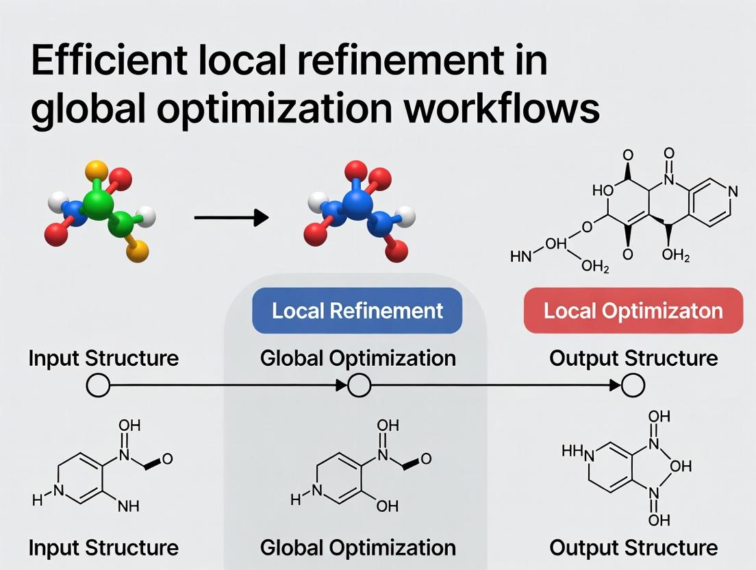
In the context of a broader thesis on Efficient local refinement in global optimization workflows, this support center addresses key technical challenges. In global optimization, a broad search space is first explored to identify promising regions. Local refinement then intensively searches these specific regions to find the precise optimal solution, balancing computational efficiency with accuracy. This is critical in fields like drug development for tasks such as molecular docking or lead optimization.

Troubleshooting Guides & FAQs

FAQ 1: During a molecular docking workflow, my global search identifies a potential binding pocket, but the subsequent local refinement fails to converge on a stable pose. What could be wrong?

• Answer: This often indicates a mismatch between the sampling algorithms or force fields used in the two phases. Ensure the local refinement protocol uses a higher fidelity scoring function or more precise conformational sampling than the global phase. Check for clashes ignored in the global screen but critical locally. Increase the number of local refinement iterations starting from the global seed points.

FAQ 2: How do I determine the optimal budget (e.g., computational time) to allocate to global search versus local refinement in my experiment?

• Answer: There is no universal rule, but a systematic approach is recommended. Start with a pilot study using a known benchmark. Allocate budgets in ratios (e.g., 70/30, 50/50, 30/70 global/local) and compare result quality. Use the data to fit a simple efficiency model. A typical starting point in many studies is a 60/40 global-to-local split.

Table: Example Budget Allocation Pilot Results for a Protein-Ligand Docking Run

Global Search Time (%)	Local Refinement Time (%)	Average Binding Affinity (kcal/mol)	Top Pose RMSD (Å)	Total Runtime (hr)
80	20	-7.2	2.5	5.0
60	40	-8.5	1.8	5.0
40	60	-8.6	1.7	5.0
20	80	-8.6	1.7	5.0

FAQ 3: My local refinement algorithm gets "stuck" in a suboptimal local minimum very close to the starting point provided by the global search. How can I encourage more exploration during refinement?

• Answer: This is a classic over-exploitation issue. Introduce mild stochasticity into your local refinement routine. Techniques include:
  • Multiple Starts: Initiate local refinement from multiple top global solutions, not just the best one.
  • Perturbation: Slightly perturb the coordinates or parameters of the seed point before beginning local optimization.
  • Hybrid Methods: Use algorithms like Basin Hopping or Lamarckian GA that allow for controlled "jumps" during local search.

Experimental Protocol: Benchmarking Local Refinement Strategies

Objective: To evaluate the efficiency of three local refinement methods following a genetic algorithm (GA) global search for molecular conformation optimization.

Materials: See "The Scientist's Toolkit" below.

Methodology:

• Global Phase: Run a standard genetic algorithm (population size=100, generations=50) to generate 10 diverse, low-energy candidate conformations.
• Refinement Phase: For each of the 10 candidates, apply three local methods in parallel:
  • A. Gradient-Based (BFGS): Perform local minimization using the BFGS algorithm until gradient tolerance < 0.01 kcal/mol/Å.
  • B. Stochastic (MC): Run a Monte Carlo Simulated Annealing protocol (1000 steps, exponential cooling).
  • C. Hybrid (Basin Hopping): Execute 50 basin hopping cycles, each comprising a random perturbation, minimization, and Metropolis criterion.
• Evaluation: Record the final energy, RMSD from the known crystal structure, and computational cost for each refined solution. Compare the best result from each method.

Workflow & Pathway Diagrams

Title: High-Level Global-Local Optimization Workflow

Title: Parallel Local Refinement of Multiple Global Candidates

The Scientist's Toolkit: Key Research Reagent Solutions

Table: Essential Materials for Computational Local Refinement Experiments

Item / Reagent	Function in Experiment	Example Vendor/Software
Molecular Dynamics (MD) Engine	Provides high-fidelity force fields for energy minimization and conformational sampling during local refinement.	GROMACS, AMBER, OpenMM
Docking & Sampling Suite	Contains algorithms for both global stochastic search (e.g., GA) and local gradient-based refinement.	AutoDock Vina, Schrödinger Glide, Rosetta
Force Field Parameter Set	Defines the energy landscape (bond, angle, dihedral, non-bonded terms) for accurate local geometry optimization.	CHARMM36, ff19SB, OPLS4
Ligand Parameterization Tool	Generates necessary bond and charge parameters for novel small molecules prior to refinement.	antechamber (AMBER), CGenFF, LigParGen
High-Performance Computing (HPC) Cluster	Enables parallel execution of multiple local refinement runs from different global starting points.	Local Slurm Cluster, AWS Batch, Google Cloud
Visualization & Analysis Software	Used to visually inspect refined poses, calculate RMSD, and analyze interaction energies.	PyMOL, UCSF ChimeraX, VMD

Technical Support Center: Troubleshooting Local Refinement in Global Drug Optimization

FAQs & Troubleshooting Guides

Q1: Our global search (e.g., using genetic algorithms) identifies a promising ligand pose, but subsequent local energy minimization collapses it into a high-energy, unrealistic conformation. What is the primary cause and solution?

A1: This is a classic symptom of inadequate force field parameterization or implicit solvent model failure during the local refinement step.

• Cause: The global search may use a simplified scoring function. The local minimizer, using a more detailed force field, encounters parameter mismatches (e.g., for a novel ligand torsional angle) or inaccurate solvation/entropic effects, pulling the pose into a locally stable but globally irrelevant well.
• Solution: Implement a multi-stage refinement protocol.
  • Initial Relaxation: Use a softened potential (e.g., GB/SA with a distance-dependent dielectric) for the first minimization steps.
  • Parameter Assignment: Ensure robust parameter derivation for novel ligand moieties using QM/MM fitting before final refinement.
  • Ensemble Refinement: Refine not a single pose, but the top-N poses (e.g., N=10) from the global search, then re-rank using binding free energy estimates (MM/PBSA, MM/GBSA).

Q2: During Hamiltonian Replica Exchange MD (H-REMD) used for local basin exploration, we observe poor exchange rates (<15%) between adjacent replicas. This hampers sampling efficiency. How do we rectify this?

A2: Poor exchange rates indicate insufficient overlap in the potential energy distributions of adjacent replicas.

• Troubleshooting Steps:
  • Check Lambda Spacing: Use a smaller difference in the coupling parameter (λ) between replicas. The number of replicas required scales with √N (degrees of freedom).
  • Adjust Hamiltonian: For alchemical transformations, ensure soft-core potentials are properly tuned to avoid singularities.
  • Diagnostic Table: Monitor potential energy overlap.

Metric	Target Value	Observed Value	Corrective Action
Replica Exchange Rate	20-30%	<15%	Increase replica count or optimize λ spacing.
Potential Energy Overlap	>0.3	<0.2	Use tools like pymbar to analyze and adjust λ schedule.
Simulation Time per Replica	>50 ps	10 ps	Increase sampling time before attempting exchange.

• Protocol: To optimize λ spacing, run a short simulation and calculate the energy variance. Use the formula for approximately constant acceptance probability: Δλ ∝ 1/√(∂V/∂λ)².

Q3: When applying a meta-dynamics simulation to escape a local energy minimum in a protein-binding pocket, the system becomes unstable. What controls are critical?

A3: Unstable dynamics typically arise from overly aggressive bias deposition or incorrect collective variable (CV) selection.

• Critical Controls:
  • CV Selection: Use at least two CVs (e.g., ligand RMSD and a specific protein-ligand distance). A single CV may force unrealistic paths.
  • Bias Parameters: Start with a height of 0.5-1.0 kJ/mol and a width 20-30% of the CV fluctuation. Deposition every 500-1000 steps.
  • Wall Potential: Apply soft harmonic walls to prevent exploration of non-physical CV values.
• Protocol:
  • Define 2-3 physically meaningful CVs.
  • Perform a short unbiased simulation to estimate CV fluctuations (σ).
  • Set Gaussian width to 0.2*σ.
  • Use a well-tempered meta-dynamics variant to control bias growth: biasfactor = 10-30.
  • Monitor CVs and protein backbone RMSD for stability.

Q4: In our FEP calculations for lead optimization, the calculated ΔΔG between two similar ligands shows high variance (>1.0 kcal/mol) between repeat windows. How can we improve precision?

A4: High variance points to insufficient sampling of conformational degrees of freedom or charge masking issues.

• Solution Guide:
  • Extended Equilibration: Equilibrate each window for >250 ps before >2 ns of production sampling.
  • Soft-Core Potentials: Ensure they are enabled for Lennard-Jones and Coulombic terms to avoid endpoint singularities.
  • Charge Transformation Protocol: For charging/discharging atoms, use a decouple/annihilate protocol in explicit solvent, not direct alchemical conversion between two charged states.

Reagent/Solution	Function in Local Refinement Context
Explicit Solvent Box (TP3P, OPC)	Models specific water-mediated interactions and entropy crucial for accurate local pose scoring.
Particle Mesh Ewald (PME)	Handles long-range electrostatic interactions accurately during MD-based refinement.
Soft-Core Potentials	Prevents singularities and numerical instabilities in alchemical FEP/REMD transformations.
Restrained Electrostatic Potential (RESP) Charges	Provides QM-derived, transferable partial charges for ligands, ensuring force field compatibility.
Linear Interaction Energy (LIE) Templates	Offers a faster, semi-empirical endpoint method for pre-screening poses before full FEP.
BioFragment Database (BFDb)	Supplies pre-parameterized fragments for novel chemotypes, reducing force field errors.

Experimental Protocol: Integrated Global-Local Pose Refinement and Scoring

Objective: To refine and accurately score the top-10 poses from a global docking run against a kinase target.

Materials: Protein structure (PDB), ligand mol2 file, AMBER/OpenMM suite, high-performance computing cluster.

Method:

• Global Docking: Perform ensemble docking with 5 receptor conformations using a genetic algorithm (e.g., GOLD).
• Pose Clustering: Cluster the top 500 poses by ligand RMSD (cutoff 2.0 Å). Select centroid of each top-10 cluster.
• System Preparation: Solvate each protein-ligand complex in an OPC water box, add ions to 0.15M NaCl.
• Local Relaxation:
  • Stage 1: Minimize with restraints on protein heavy atoms (force constant 5.0 kcal/mol/Ų).
  • Stage 2: Minimize with restraints on protein backbone only.
  • Stage 3: Full minimization (no restraints).
• Equilibration: NVT (100 ps, 298 K) → NPT (200 ps, 1 atm, 298 K).
• Production & Scoring: Run 5 ns MD per pose. Calculate MM/GBSA ΔG from 1000 evenly spaced frames. Perform statistical analysis (mean, SEM).

Workflow: Integrated Global-Local Pose Optimization

Meta-Dynamics Enhanced Sampling Mechanism

Technical Support Center: Troubleshooting & FAQs

General Workflow Optimization

Q1: My multi-start heuristic is converging to sub-optimal local minima despite numerous starts. What systemic issue might be at play? A: This is often a problem of insufficient diversification in your initial sampling strategy. Ensure your starting points are generated via a Low-Discrepancy Sequence (e.g., Sobol sequence) or a well-tuned Latin Hypercube Sampling instead of pure pseudo-random numbers. For problems with n dimensions, a minimum of 10n to 50n starting points is typically required for complex energy landscapes. Check the spread of your final solutions; if they cluster in fewer than 3 distinct regions, your sampling is inadequate.

Q2: In a two-stage strategy, how do I determine the optimal handoff point from the global to the local solver? A: The handoff is optimal when the cost of continued global search outweighs the expected refinement benefit. Implement a convergence monitor on the global phase. A practical rule is to trigger handoff when, over the last k iterations (k = 50-100), the improvement in the best-found objective value is less than a threshold ε (e.g., 1e-4). See Table 1 for metrics.

Table 1: Two-Stage Handoff Decision Metrics

Metric	Calculation	Recommended Threshold
Relative Improvement	(f_best(iter-i) - f_best(iter))/(1e-10 + |f_best(iter)|)	< 1e-4 for 50 consecutive iterations
Solution Cluster Radius	Std. dev. of top 10 solutions' parameters	< 0.05 * (Param Upper Bound - Lower Bound)
Solver Effort Ratio	(Global_Solver_Time) / (Estimated_Local_Refinement_Time)	> 5.0

Q3: When using an embedded refinement strategy, my local search is causing computational bottlenecks. How can I mitigate this? A: This indicates your refinement is too frequent or too expensive. Implement adaptive embedded refinement:

• Trigger Condition: Only refine a solution if it is a promising basin candidate (e.g., its objective value is within the top 15% of all candidates in the current generation/population).
• Budget Limiter: Cap the number of local iterations (e.g., 50-100 gradient steps) or function evaluations per refinement call.
• Memoization: Cache refined solutions to avoid redundant local searches from similar starting points.

Experiment-Specific Protocols

Protocol 1: Benchmarking Multi-Start Strategies for Molecular Docking This protocol assesses the efficiency of different multi-start configurations in finding low-binding-energy poses.

• System Preparation: Prepare the protein receptor (fixed) and ligand (flexible) files in PDBQT format using AutoDock Tools.
• Parameter Space Definition: Define the search space (translational, rotational, torsional).
• Multi-Start Execution:
  • Run Vina or AutoDock-GPU with exhaustiveness = N, where N is the number of starts (e.g., 8, 16, 32, 64).
  • For each N, perform 10 independent runs to account for stochasticity.
• Data Collection: Record the best binding affinity (kcal/mol) and runtime for each run.
• Analysis: Plot the best-found affinity vs. exhaustiveness and runtime vs. exhaustiveness. The optimal N is at the knee of the curve where affinity gains diminish relative to time cost.

Protocol 2: Two-Stade Optimization for Force Field Parameterization This protocol uses a global metaheuristic followed by local gradient-based refinement to fit parameters.

• Stage 1 - Global Exploration:
  • Use a Differential Evolution (DE) algorithm. Population size = 10 * number of parameters.
  • Termination: After 200 generations or if population diversity (norm of std. dev. of parameters) < 1e-3.
  • Output: The top 5 parameter vectors from the final population.
• Stage 2 - Local Refinement:
  • For each parameter vector from Stage 1, initiate a Levenberg-Marquardt optimizer.
  • Objective: Minimize the weighted sum of squared errors between calculated and experimental observables (e.g., bond lengths, angles, energies).
  • Termination: On gradient norm < 1e-5 or 500 iterations.
• Validation: Select the overall best-refined parameter set and validate on a held-out set of experimental data.

Visualizing Strategies

The Scientist's Toolkit: Research Reagent Solutions

Table 2: Essential Tools for Optimization Experiments

Item	Function in Optimization Workflow	Example Product/Software
Global Solver	Executes the high-level search (Multi-Start, Evolutionary, etc.) to explore the solution space broadly.	NLopt (DIRECT, CRS2), SciPy (differential_evolution), OpenMDAO.
Local Refiner	Performs intensive, convergent search from a given starting point to find a local minimum.	IPOPT, L-BFGS-B (SciPy), SNOPT, gradient descent in PyTorch/TensorFlow.
Surrogate Model	Provides a cheap-to-evaluate approximation of the objective function to guide sampling.	Gaussian Process (GPyTorch, scikit-learn), Radial Basis Functions.
Sampling Library	Generates high-quality initial points or search directions for multi-start or population methods.	Sobol Sequence (SALib), Latin Hypercube (PyDOE), Halton Sequence.
Benchmark Suite	Provides standardized test problems to validate and compare optimization strategy performance.	CUTEst, COCO (Black-Box Optimization), molecular docking benchmarks (PDBbind).
Convergence Analyzer	Monitors iteration history to automatically detect stagnation for handoff or termination decisions.	Custom scripts using metrics from Table 1; Optuna's visualizations.
Parallelization Framework	Manages concurrent evaluation of multiple starts or population members to reduce wall-clock time.	MPI (mpi4py), Python's multiprocessing, Ray, Dask.

This technical support center provides guidance for researchers implementing optimization workflows within drug discovery and related fields. The content is framed within the broader research thesis on Efficient local refinement in global optimization workflows, addressing common challenges in balancing global exploration with local exploitation.

Troubleshooting Guides & FAQs

FAQ 1: How do I know if my optimization is stuck in a local optimum prematurely?

Answer: Monitor the "Improvement Rate" metric. A sustained period (e.g., 20 consecutive iterations) with less than 0.5% improvement in your objective function, while global uncertainty (measured by sample variance in unexplored regions) remains high, suggests premature exploitation. Implement a checkpoint to trigger a secondary, exploratory sampling protocol.

FAQ 2: What is a practical metric to quantify the exploration-exploitation balance in real-time?

Answer: Use the Global vs. Local Acquisition Ratio (GLAR). Calculate the ratio of resources (e.g., computational budget, experimental batches) dedicated to global search versus local refinement over a sliding window. The target ratio is problem-dependent but should be explicitly defined.

Table: Key Metrics for Balance Monitoring

Metric	Formula/Description	Target Range (Typical)	Indicates Imbalance When...
Improvement Rate	(fbest(t) - fbest(t-n)) / n	>1% per n iters. (Adaptive)	Consistently near zero.
GLAR	(Budget on Global) / (Budget on Local)	70/30 to 30/70 (Early/Late)	Stays >80/20 or <20/80.
Region Uncertainty	Avg. predictive variance of model in top N regions.	Relative to initial variance.	High but unexplored.
Diversity Score	Avg. distance between proposed samples.	Maintain >X% of initial score.	Clusters too tightly.

FAQ 3: My local refinement step fails to improve the best-found candidate. How should I troubleshoot?

Answer: Follow this protocol:

• Verify Fidelity: Ensure your local surrogate model or experimental assay has sufficient precision. Re-run the current best point to confirm its performance.
• Check Gradient Reliability: If using model-based gradients, verify them against finite-difference approximations in a small neighborhood.
• Expand Refinement Radius: Temporarily increase the trust region or local search boundary by 50%. If improvement appears, the local basin is wider than estimated.
• Escalate to Hybrid: Trigger a "global-informed local" step: perform a short exploratory search focused on the most promising other region before returning to refine the current best.

FAQ 4: How do I set the iteration budget between global and local phases?

Answer: Use an adaptive schedule based on Expected Global Potential (EGP). EGP estimates the possible improvement in unexplored spaces versus expected local improvement. Switch phases when EGP for global exceeds that for local by a set threshold (e.g., 1.2x).

Experimental Protocols

Protocol: Iterative Optimization Cycle with Adaptive Switching

Purpose: To systematically balance exploration and exploitation in a computationally efficient manner. Methodology:

• Initialization: Perform a space-filling design (e.g., Latin Hypercube) for N initial samples (N = 10 * dimensionality).
• Model Training: Fit a global surrogate model (e.g., Gaussian Process, Random Forest) to all data.
• Phase Decision (Adaptive Switch):
  • Calculate the Exploitation Score (ES): Predicted improvement from refining the current top 3 candidates.
  • Calculate the Exploration Score (ER): Maximum predictive uncertainty across M random untested points.
  • If ER / ES > threshold (θ), proceed to Global Phase. Else, proceed to Local Phase.
• Global Phase: Use an acquisition function (e.g., Expected Improvement, Upper Confidence Bound) to select the next batch of 3-5 points from the entire space.
• Local Phase: Apply a trust-region method (e.g., DIRECT, BOBYQA) or a local Gaussian Process refinement focused on the best candidate's region to select the next 1-2 points.
• Evaluation & Update: Run experiments/simulations for the proposed points, update the dataset, and return to Step 2. Terminate after budget exhaustion or convergence.

Protocol: Calibrating the Balance Threshold (θ)

Purpose: To empirically determine the optimal switching threshold for a specific class of problems. Methodology:

• Select 2-3 representative benchmark functions or historical datasets with known optima.
• Run the Iterative Optimization Cycle (above) 50 times per candidate threshold value (θ = [1.0, 1.5, 2.0, 3.0]).
• Record the final best objective value and the iteration at which the true optimum was first approximated within 5%.
• Analysis: Plot θ against both the final performance and the speed of convergence. The optimal θ minimizes convergence time without degrading final performance. Use this value for subsequent similar experiments.

Visualizations

Diagram: High-Level Optimization Workflow with Adaptive Switch

Diagram: Key Metrics Feedback to Phase Decision

The Scientist's Toolkit: Research Reagent Solutions

Table: Essential Materials for Optimization Workflow Experiments

Item / Reagent	Function in Context	Example & Notes
Global Surrogate Model	Approximates the expensive objective function across the entire input space for prediction and uncertainty quantification.	Gaussian Process (GP) with Matérn kernel. Note: Use scalable approximations (e.g., sparse GP) for high dimensions.
Local Solver / Refiner	Performs intense search within a constrained region (trust region) to converge to a local optimum.	BOBYQA (Bound Optimization BY Quadratic Approximation). Note: Effective for derivative-free, constrained local refinement.
Acquisition Function	Balances exploration and exploitation by proposing the next most valuable point(s) to evaluate.	q-EI (Batch Expected Improvement). Note: Enables parallel, batch experimental design.
Adaptive Threshold (θ)	A calibrated parameter that controls the switch between global and local phases based on ER/ES ratio.	Determined via Protocol: Calibrating the Balance Threshold. Start with θ=1.5.
Benchmark Suite	Validates the optimization workflow's performance on problems with known solutions.	Synthetic: Branin, Hartmann functions. Industrial: Pharma QSAR datasets with published binding affinities.
High-Throughput Assay	The experimental system used to evaluate the objective function (e.g., binding affinity, yield).	Example: Fluorescence-based binding assay in 384-well plates. Critical for throughput.

Implementing Local Refinement: Algorithms and Real-World Applications

Technical Support Center

Troubleshooting Guides & FAQs

Q1: My gradient-based optimizer (e.g., L-BFGS-B) is converging to a poor local minimum from the starting point provided by my global search. What are the primary checks? A: This is a common issue in the refinement phase. Follow this protocol:

• Check Gradient Fidelity: Use finite-difference checks at the global solution seed point. Discrepancies >1e-6 suggest an error in the objective or gradient function implementation.
• Evaluate Starting Point Feasibility: Ensure the point satisfies all bound and nonlinear constraints. Infeasible starts can cause immediate failure.
• Adjust Optimizer Tolerance: For refinement, tighten factr (L-BFGS-B) or gtol parameters. Suggested: factr=1e10 (moderate) to 1e12 (tight).
• Implement Multi-Start Refinement: Automate the launch of the local optimizer from the top N (e.g., 5-10) solutions of the global search, not just the best.

Q2: My quasi-Newton method fails with "non-positive definite Hessian" errors during molecular geometry optimization. How to resolve? A: This indicates ill-conditioning, often near saddle points or with numerical noise.

• Initial Hessian Strategy: Do not use a unit matrix. Use a scaled diagonal or, better, a calculated Hessian from a lower-level theory (e.g., MMFF94) for the initial guess.
• Trust-Region Enforcement: Use a trust-region method (e.g., trust-constr in SciPy) instead of line-search. It handles indefinite Hessians robustly.
• Switch to Gradient-Only: As a diagnostic, temporarily use a gradient-only method (e.g., nonlinear conjugate gradient). If it proceeds, the issue is Hessian approximation.
• Regularization: Add a small Levenberg-Marquardt damping term (lambda * I) to the Hessian update to enforce positive definiteness.

Q3: The surrogate model (e.g., Gaussian Process) in my optimization loop is inaccurate, leading to failed local refinements. How to improve it? A: Surrogate inaccuracy often stems from poor training data or hyperparameters.

• Active Learning for Refinement: In the local basin, enrich the surrogate training set with points from a Design of Experiment (DoE) around the best point before refinement. A spherical LHS with radius=0.2*norm(globalsearchrange) is effective.
• Hyperparameter Re-Optimization: Re-optimize GP kernel scales and noise parameters using MLE after the global phase and before local refinement.
• Hybrid Objective: For refinement, use a weighted sum of surrogate mean and standard deviation (Expected Improvement) to balance exploitation and exploration locally.
• Dimensionality Check: For >20 dimensions, consider using partial dependence plots to check if the surrogate has captured variable sensitivities.

Q4: How do I balance computational cost between global exploration and local refinement when optimizing a costly molecular property? A: This is the core of efficient workflow design. Implement an adaptive budget allocator.

Table 1: Comparative Performance of Local Methods for Refinement (Hypothetical Benchmark)

Method	Avg. Function Calls to Converge	Success Rate (%)	Avg. Final Objective Improvement	Best For
BFGS (Gradient)	45	85	15.2%	Smooth, low-dim problems
L-BFGS-B (Gradient)	55	92	14.8%	Bounded, medium-dim problems
SLSQP (Gradient)	65	88	16.1%	Constrained problems
DFP (Quasi-Newton)	50	82	14.9%	Historical comparison
Surrogate-Assisted (EI)	20 (surrogate) + 3 (true)	95	17.5%	Very expensive objectives

Experimental Protocol for Benchmarking Refinement Methods

• Objective: Compare the efficiency of local refinement methods post-global search.
• Procedure:
  • Run a differential evolution global search for 1000 iterations on a test suite (e.g., 10 shifted Schwefel functions). Record the top 5 candidate solutions.
  • For each local method (BFGS, L-BFGS-B, SLSQP), initialize from each of the 5 candidates with identical, tight tolerance settings (gtol=1e-9).
  • For the surrogate-assisted method, build a GP model on the final 200 points from the global search. Refine the best point using the EI criterion, validating with a true function call every 5 surrogate steps.
  • Measure: number of true function calls to reach gtol, final objective value, and success (convergence within max iterations).
• Key Parameters: Population size=50, CR=0.9, F=0.8 (DE). GP kernel=Matern 5/2. Max local iterations=200.

Title: Hybrid Global-Local Optimization Workflow

The Scientist's Toolkit: Research Reagent Solutions

Table 2: Essential Toolkit for Optimization Experiments

Item / Solution	Function in the "Experiment"	Example / Specification
Global Optimizer	Provides diverse starting points for local refinement.	Differential Evolution (SciPy), Bayesian Optimization (Ax), CMA-ES.
Gradient Calculator	Supplies 1st-order info for gradient-based methods.	Automatic Differentiation (JAX, PyTorch), Adjoint Solvers, Finite Differencing.
Hessian Approximator	Builds 2nd-order model for quasi-Newton methods.	BFGS, SR1, or L-BFGS update routines (from SciPy, NLopt).
Surrogate Model	Creates a cheap-to-evaluate proxy of the expensive objective.	Gaussian Process (GPyTorch, scikit-learn), Radial Basis Functions.
Convergence Monitor	Tracks progress and decides termination of refinement.	Custom logger checking `|	grad		< gtolandΔf < ftol` over window.
Benchmark Problem Set	Validates and compares the performance of the full toolkit.	COBYLA, Shifted-Schwefel, or proprietary molecular property functions.

Title: Information Flow in a Local Refinement Step

Technical Support Center

Troubleshooting Guide

Issue T1: Solver Handoff Failure

• Symptoms: The global solver completes its run, but the local solver does not initiate. The workflow halts or errors with a "boundary condition not met" message.
• Diagnosis: This is typically a data formatting or interface mismatch. The output from the global solver (e.g., a candidate solution vector, basin identifier) is not in the precise format or structure expected by the local solver's input API.
• Resolution:
  • Implement a validation and translation layer (an "adapter") between the solvers.
  • Log the exact output of the global solver and compare it to the expected input schema of the local solver.
  • Ensure numerical precision (e.g., single vs. double) and parameter bounds are explicitly passed and respected.

Issue T2: Premature Convergence or Cycling

• Symptoms: The coupled system converges to a suboptimal solution or appears to oscillate between a few points without refining.
• Diagnosis: Inadequate criteria for triggering the switch from global exploration to local refinement. The handoff may be happening too early (before the global basin is identified) or the local solver is being called repeatedly on the same region.
• Resolution:
  • Implement and tune a robust handoff criterion. Common metrics are listed in Table 1.
  • Introduce a tabu or caching mechanism to prevent the global solver from revisiting and re-submitting recently refined regions.

Issue T3: Prohibitive Computational Overhead

• Symptoms: The overall runtime of the coupled system is much higher than the sum of isolated solver runtimes, negating the benefit of integration.
• Diagnosis: Excessive communication overhead (e.g., file I/O, process spawning) or an inefficient parallelization strategy between the global and local components.
• Resolution:
  • Shift from file-based to memory-based (e.g., shared, message-passing) inter-process communication.
  • Use a lightweight, persistent local solver instance that can be warm-started, rather than launching a new process for each refinement task.

Frequently Asked Questions (FAQs)

Q1: What is the most critical parameter to configure in a coupled architecture? A1: The handoff criterion. This logic determines when and where to invoke the local solver based on the global solver's progress. A poorly set criterion is the primary cause of inefficiency or failure in integrated workflows.

Q2: Can I couple a gradient-based local solver with a derivative-free global solver? A2: Yes, this is a common and powerful pattern. The key is to ensure the global solver provides a sufficiently refined starting point within the convergence basin of the local solver. You may need to configure the local solver with conservative initial step sizes to bridge the fidelity gap.

Q3: How do I manage different levels of model fidelity between solvers? A3: Implement a surrogate or proxy model. Use a fast, lower-fidelity model (e.g., coarse-grid, molecular mechanics) for the global explorer. When a promising region is identified, switch to a high-fidelity model (e.g., all-atom, quantum mechanics) for the local refinement. Calibration between model fidelities is essential.

Q4: What are the best practices for parallelizing such a workflow? A4: Employ an asynchronous master-worker pattern. The global solver (master) continuously proposes candidate points. Idle workers request these points and conduct local refinements in parallel. Results are asynchronously fed back to inform the global search, preventing bottlenecks.

Data & Methodology

Table 1: Common Handoff Criteria for Solver Coupling

Criterion	Metric Description	Best For	Typical Threshold Range
Population Cluster Density	Coefficient of variation of candidate points in a promising region.	Population-based global solvers (e.g., GA, PSO).	Variance < 0.1 * Search Space
Trust Region Radius	Size of the region around the best candidate where a local model is trusted.	Surrogate-assisted or Bayesian optimization.	Radius < 5-10% of domain
Probability of Improvement	Likelihood that a candidate point will outperform the current best.	Bayesian Optimization frameworks.	PoI > 0.15
Gradient Estimate Norm	Magnitude of an estimated gradient (finite difference) at the candidate point.	Heuristic link to gradient-based local search.	||Gradient| < 1e-3

Experimental Protocol: Benchmarking Coupled Architectures

Objective: Quantify the efficiency gain of a coupled Global-Local solver versus a standalone global solver for molecular conformation search.

• Problem Set: Select 5 small organic molecules with known conformational energy landscapes (e.g., from PubChem).
• Solver Setup:
  • Global: Stochastic algorithm (e.g., Particle Swarm Optimization) using an MMFF94 force field.
  • Local: Gradient-based algorithm (e.g., L-BFGS) using the same or a higher-fidelity (DFT) method.
  • Coupling: Implement a handoff when the PSO cluster density criterion (Table 1) is met.
• Execution: For each molecule, run (a) Global-only for 10,000 iterations, and (b) Coupled system with a handoff budget of 200 local iterations.
• Metrics: Record the best energy found and wall-clock time to reach within 5% of the known global minimum. Average results over 20 independent runs to account for stochasticity.

Visualizations

Diagram Title: Basic Synchronous Coupling Workflow

Diagram Title: Asynchronous Master-Worker Parallel Architecture

The Scientist's Toolkit: Research Reagent Solutions

Item	Function in Integration Experiments
Optimization Framework (e.g., Pyomo, SciPy)	Provides the scaffolding to define objective functions, constraints, and manage solver interfaces.
Message Passing Interface (MPI)	Enables high-performance, parallel communication between globally distributed and locally focused solver processes.
Surrogate Model Library (e.g., scikit-learn, GPyTorch)	Used to build fast approximate models (Gaussian Processes, Neural Networks) for the global exploration phase.
Containerization (Docker/Singularity)	Ensures solver environment consistency and portability across HPC clusters, crucial for reproducible workflows.
Molecular Mechanics Force Field (e.g., OpenMM)	Acts as the fast, lower-fidelity "global" evaluator for conformational search in drug development.
Quantum Chemistry Package (e.g., PySCF, ORCA)	Acts as the high-fidelity "local" refiner for accurate electronic energy calculations.
Data Serialization (Protocol Buffers, HDF5)	Enables efficient, language-agnostic data transfer of complex candidate solutions between solver components.

Troubleshooting Guides & FAQs

Q1: During a global optimization run, my algorithm fails to trigger local refinement even when it appears to have entered a promising parameter basin. What are the primary criteria checks that might be failing?

A: The failure to trigger local refinement is typically due to one or more of the following criteria not being met. Verify these conditions sequentially:

• Basin Stability Criterion: The point must reside within a region of parameter space where the objective function value has shown consistent improvement or minimal fluctuation (low variance) over a defined number of consecutive iterations (N_stable). A common failure is a too-short stability window.
• Gradient Norm Threshold: While not always computed in derivative-free global methods, proxy gradient estimates (e.g., from simplex vertices or recent steps) may be used. The norm must fall below a set threshold (ε_grad). Check if your threshold is too strict.
• Significant Improvement Criterion: The candidate point must represent an improvement over the current best solution by a margin greater than a noise tolerance level (Δ_significant). This prevents refinement on statistically insignificant fluctuations.
• Resource Budget Check: Local refinement may be withheld if the allocated budget (e.g., function evaluations, time) for the global phase is exhausted or if the remaining budget is insufficient for a minimum local refinement run.

Q2: What are robust experimental protocols for validating basin detection and refinement triggers in a synthetic test environment?

A: Follow this detailed protocol to validate your triggering logic:

Protocol: Validation of Refinement Triggers on Synthetic Functions

• Preparation: Select a set of standard benchmark functions with known basin locations (e.g., Rosenbrock, Rastrigin, Ackley functions).
• Instrumentation: Modify your global optimization algorithm to log all proposed trigger points, the state of all triggering criteria at that iteration, and the final decision (trigger/not trigger).
• Ground Truth Labeling: For each iteration, determine if the current solution is actually within a predefined radius (r_basin) of a known global/local minimum (ground truth basin).
• Run Experiments: Execute multiple optimization runs on the benchmark set. Record all data.
• Analysis: Calculate the True Positive Rate (correct triggers inside true basins) and False Positive Rate (erroneous triggers outside true basins) for your criteria. Adjust criterion thresholds to optimize this balance.

Q3: How do I quantify the efficiency gain from an adaptive local refinement trigger versus a fixed-interval schedule?

A: The efficiency gain is measured by comparing resource consumption to reach a target solution quality. Conduct the following comparative experiment:

Protocol: Comparative Efficiency Measurement

• Control Group: Run your optimization workflow with a fixed-interval local refinement schedule (e.g., trigger every K iterations).
• Test Group: Run the same workflow with your adaptive basin-detection trigger.
• Metrics: For both groups, record the total number of function evaluations and computational time required for the best-found solution to reach a pre-specified objective value threshold (V_target).
• Calculation: Compute the percentage reduction in evaluations and time for the test group versus the control. Statistical significance should be assessed using multiple independent runs.

Table 1: Example Quantitative Results from a Benchmark Study (Hypothetical Data)

Benchmark Function	Fixed-Trigger Evaluations (Mean)	Adaptive-Trigger Evaluations (Mean)	Reduction in Evaluations	Probability of Successful Trigger (True Positive)
Rosenbrock (2D)	15,750	9,420	40.2%	92%
Rastrigin (5D)	52,300	38,950	25.5%	85%
Ackley (10D)	121,000	110,200	8.9%	78%

Workflow & Logical Diagram

Title: Logical Flow for Triggering Local Refinement

The Scientist's Toolkit: Research Reagent Solutions

Table 2: Essential Components for a Hybrid Optimization Workflow

Item	Function/Explanation
Global Optimizer (e.g., CMA-ES, Bayesian Optimization)	Explores the broad parameter space to identify promising regions, avoiding premature convergence to local minima.
Local Refinement Solver (e.g., L-BFGS, Nelder-Mead)	Once a basin is detected, this efficient local algorithm converges rapidly to the precise local minimum.
Basin Detection Module	Contains the logic (criteria) for analyzing the optimizer's trajectory to signal a potential convergence basin.
Benchmark Function Suite	Synthetic landscapes with known properties for validating trigger accuracy and algorithm performance.
Performance Metrics Logger	Tracks key data (evaluations, time, objective value) to quantify the efficiency gains of the adaptive trigger.

Troubleshooting Guides & FAQs

Q1: During conformer generation, my workflow stalls with the error "Failed to generate low-energy conformers." What are the primary causes? A: This typically indicates an issue with the input geometry or parameterization. First, verify the initial 3D structure is valid (no atomic clashes, reasonable bond lengths). Second, ensure the correct force field (e.g., MMFF94s, GAFF2) is applied for your molecule type (small organic vs. metallocomplex). Third, increase the maximum iteration limit for the energy minimization step. A protocol adjustment is to first perform a coarse conformational search using a faster method (e.g., ETKDG) followed by local refinement with the more precise force field.

Q2: The docking scores from my locally refined poses show high variance (>3 kcal/mol) between repeated runs on the same protein-ligand pair. How can I stabilize the results? A: High variance suggests insufficient sampling during the local refinement stage. Implement the following: 1) Increase the number of refinement steps (e.g., from 50 to 200 in the local optimizer). 2) Apply a stronger conformational restraint on the protein's backbone during ligand pose refinement to prevent unnatural protein drift. 3) Use a consistent and reproducible random seed for the optimization algorithm. The core thesis of efficient local refinement emphasizes balancing sampling depth with computational cost; a slight increase in refinement iterations often stabilizes scores without major time penalties.

Q3: After local refinement of docked poses, the ligand is distorted with unusual bond angles. What went wrong? A: This is a failure in the force field's bonded parameters or an over-aggressive optimization. Apply this protocol: First, check that the ligand was correctly parameterized (atom types assigned correctly). Second, in the local refinement script, increase the weight of the bonded terms (bonds, angles, dihedrals) relative to the non-bonded (vdW, electrostatic) terms in the scoring function. This ensures molecular integrity is prioritized during the local search.

Q4: How do I quantify the improvement from adding a local refinement step to my global docking pipeline? A: You must compare key metrics with and without refinement. Run your standard global docking (e.g., Vina, QuickVina 2) on a benchmark set, then apply your local refinement (e.g., using OpenMM for minimization). Compare the results as shown in Table 1.

Table 1: Docking Performance Metrics With vs. Without Local Refinement

Metric	Global Docking Only	Global + Local Refinement	Measurement Protocol
RMSD to Crystal Pose (Å)	2.5 ± 0.8	1.2 ± 0.4	Calculate after aligning protein backbone.
Average Docking Score (kcal/mol)	-7.1 ± 1.5	-8.9 ± 1.2	More negative scores indicate stronger predicted binding.
Pose Ranking Accuracy (%)	65%	89%	% of cases where top-ranked pose is <2.0 Å RMSD to crystal.
Computational Time (sec/ligand)	45 ± 10	68 ± 12	Measured on a standard CPU node.

Experimental Protocol for Benchmarking:

• Dataset Preparation: Select the PDBbind core set (or a relevant subset of 50-100 protein-ligand complexes with high-resolution crystal structures).
• Global Docking: For each complex, separate the ligand, generate 10 conformers, and dock into the prepared protein binding site using your chosen global method (e.g., exhaustiveness=32 in Vina). Save the top 10 poses.
• Local Refinement: For each of the top 10 global poses, perform a local energy minimization. Protocol: Use the OpenMM toolkit with the AMBER ff14SB force field for the protein and GAFF2 for the ligand. Solvate implicitly (GBSA). Run 1000 steps of steepest descent minimization.
• Re-scoring: Score the refined poses using the same scoring function as the global docker for fair comparison.
• Analysis: For each complex, identify the pose with the best score after refinement. Calculate its RMSD to the crystal ligand pose. Aggregate statistics across the entire dataset.

Q5: My locally refined poses cluster into very similar conformations, suggesting a lack of diversity. How can I maintain diversity while improving accuracy? A: This is a key challenge in efficient local refinement. To address it, modify your workflow to apply local refinement to a broader set of initial poses (e.g., top 20 instead of top 5) and incorporate a diversity filter post-refinement. Cluster the refined poses by RMSD and select the best-scoring pose from each major cluster. This aligns with the thesis of using local refinement to polish multiple promising regions identified by the global search.

Diagram: Workflow for Diverse & Accurate Pose Refinement

The Scientist's Toolkit: Research Reagent Solutions

Table 2: Essential Materials for Conformer Search & Docking Experiments

Item/Software	Function & Application	Key Consideration
RDKit	Open-source cheminformatics toolkit for ligand preparation, conformer generation (ETKDG), and basic molecular operations.	The default ETKDG algorithm is fast but may require parameter tuning (numConfs) for complex macrocycles.
Open Babel / Gypsum-DL	Used for standardizing molecular formats, generating protonation states, and tautomers at a specified pH.	Critical for preparing a realistic, enumerative set of ligand states before docking.
OpenMM	High-performance toolkit for molecular dynamics and energy minimization. Used for local pose refinement with explicit force fields.	Allows precise control over the refinement protocol (steps, constraints, implicit solvent model).
AutoDock Vina / QuickVina 2	Widely-used global docking engines for rapid sampling of the protein's binding site.	Serves as the initial, broad sampling stage. Exhaustiveness parameter directly impacts initial pose quality.
AMBER/GAFF or CHARMM/CGenFF	Force field parameter sets for proteins and small molecules, providing the energy terms for local refinement.	Choice depends on system compatibility; GAFF2 is broadly applicable for drug-like ligands.
PDBbind Database	Curated collection of protein-ligand complexes with binding affinity data, used for method validation and benchmarking.	The "core set" is the standard for rigorous accuracy testing against known crystal structures.

Diagram: Thesis Context of Local Refinement in Optimization

Technical Support Center

Troubleshooting Guides & FAQs

Q1: During pose refinement, my simulation crashes with the error "NaN (not a number) detected in forces." What are the common causes and solutions? A: This typically indicates an instability in the molecular dynamics (MD) engine.

• Cause 1: Overlapping atoms due to a poor initial pose or bad van der Waals parameters.
  • Solution: Re-center the ligand in the binding site with a small initial minimization step. Use a soft-core potential during the initial equilibration phase.
• Cause 2: Incorrectly assigned protonation states at the chosen simulation pH.
  • Solution: Use a tool like PROPKA to re-calculate protonation states of protein residues (especially Asp, Glu, His, Lys) before system preparation. Ensure ligand protonation is correct.
• Cause 3: An unstable covalent bond parameter for a modified residue or ligand.
  • Solution: Check the force field assignment. For non-standard residues/ligands, validate parameters with QC methods before simulation.

Q2: My calculated relative binding free energy (ΔΔG) between two similar ligands has an error > 2.0 kcal/mol, which is unusable. What steps should I take to debug? A: High error suggests poor phase space overlap or sampling insufficiency.

• Step 1 - Check Lambda Schedule: For alchemical transformations with large structural changes, increase the number of intermediate λ windows (e.g., from 12 to 20), especially near end-states (λ=0.0 and λ=1.0).
• Step 2 - Analyze Overlap: Plot the potential energy difference distributions between adjacent λ windows. Poor overlap appears as separate peaks.
  • Protocol: Use analysis tools (e.g., alchemical-analysis.py) to generate the overlap matrix. If off-diagonal elements are near zero, sampling is insufficient or the schedule is wrong.
• Step 3 - Extend Sampling: Increase simulation time per λ window. A good starting point is 5 ns per window for complex and solvent legs. For difficult transformations, 10-20 ns may be required.

Q3: After running an ensemble of refinements, how do I choose the final "best" pose when scores conflict (e.g., MM/GBSA suggests Pose A, but the binding pocket hydration analysis suggests Pose B)? A: Implement a consensus decision protocol.

• Cluster the Poses: Cluster refined poses by RMSD (e.g., 2.0 Å cutoff).
• Apply Multi-Metric Scoring: Create a ranked table for each cluster representative.
• Prioritize Experimental Data: If a crystallographic water network is known, the pose that best accommodates it is preferred.
• Perform a Brief Unbiased Simulation: Run a short (50-100 ns) unbiased MD of the top contenders. The pose with greater stability (lower RMSD) and more persistent key interactions is favored.

Q4: In the context of global optimization workflows, when should I use fast VSGB 2.0 scoring versus more rigorous but slower PMF-based refinement? A: The choice is a trade-off between throughput and accuracy, dependent on the workflow stage.

Workflow Stage	Sample Size	Recommended Method	Typical Compute Time per Pose	Purpose
Pre-screening	1,000 - 10,000	Fast Docking & MM/GBSA (VSGB)	2-10 minutes	Filter to top 50-100 candidates.
Local Refinement	10 - 100	MM/GBSA (VSGB 2.0) with MD	1-4 hours	Rank poses, assess interaction stability.
High-Confidence	1 - 10	Alchemical (PMF) Methods (TI, FEP)	24-72 hours	Quantitative ΔΔG for lead optimization.

Experimental Protocols

Protocol 1: MM/GBSA Refinement with Explicit Solvent Sampling This protocol refines docked poses and estimates binding affinity.

• System Preparation: Use tleap (Amber) or pdb2gmx (GROMACS) to solvate the protein-ligand complex in an orthorhombic water box (10 Å buffer), add ions to neutralize, and optionally add 150 mM NaCl.
• Minimization & Equilibration:
  • Minimize solvent and ions with protein-ligand heavy atoms restrained (500 steps steepest descent, 500 conjugate gradient).
  • Heat system from 0 K to 300 K over 100 ps in NVT ensemble with restaints.
  • Equilibrate density at 300 K/1 bar over 200 ps in NPT ensemble.
  • Release restraints over 500 ps of NPT equilibration.
• Production MD: Run an unrestrained MD simulation for 20-50 ns. Use a 2 fs timestep, PME for electrostatics, and maintain temperature/pressure with a Langevin thermostat and Berendsen barostat.
• Trajectory Sampling & MM/GBSA: Extract snapshots every 100 ps from the last 10 ns. For each snapshot, calculate the binding free energy using the MM/GBSA model (e.g., MMPBSA.py in AmberTools). The VSGB 2.0 solvation model is recommended.

Protocol 2: Relative Binding Free Energy (RBFE) Calculation using Thermodynamic Integration (TI) This protocol calculates ΔΔG for two ligands (LigA -> LigB).

• Topology Preparation: Create dual-topology hybrid structures for the ligand in complex and in solvent. Ensure proper mapping of atoms between LigA and LigB.
• Lambda Scheduling: Define a set of 12-24 λ values for coupling both electrostatic and Lennard-Jones interactions. Use a non-linear schedule (e.g., lambda_powers = 2) to place more points near end-states.
• Simulation at Each Lambda:
  • For each λ window, minimize, equilibrate (as in Protocol 1), and run production MD (2-5 ns per window).
  • Use a soft-core potential for Lennard-Jones interactions to avoid endpoint singularities.
• Analysis: For each λ window, calculate the ensemble average of dV/dλ. Numerically integrate (∫ <dV/dλ> dλ) over λ using the trapezoidal rule or Simpson's method. ΔΔGbind = ΔGcomplex - ΔG_solvent. Estimate statistical error using bootstrapping.

Diagrams

Global Optimization with Local Refinement Workflow (73 chars)

Troubleshooting High FEP/TI Error (45 chars)

The Scientist's Toolkit: Research Reagent Solutions

Item	Function & Rationale
AMBER/GAFF Force Fields	Provides parameters for organic drug-like molecules (GAFF) and standard bio-polymers (ff19SB). Essential for consistent MD and free energy calculations.
VSGB 2.0 Solvation Model	A fast, implicit solvation model with good accuracy for MM/GBSA, enabling rapid scoring of refined poses from MD trajectories.
Hydrogen Mass Repartitioning (HMR)	Allows a 4 fs MD timestep by increasing the mass of hydrogen atoms, significantly accelerating conformational sampling without loss of accuracy.
Soft-Core Potential	Prevents simulation instabilities (NaNs) in alchemical calculations by removing singularities in the Lennard-Jones potential when atoms are created/annihilated.
Orthorhombic TIP3P Water Box	The standard explicit solvent environment for hydration. A 10-12 Å buffer ensures the protein is fully solvated and minimizes periodic boundary artifacts.
Multi-Ensemble Thermostat (e.g., Langevin)	Maintains correct temperature distribution and aids sampling by introducing stochastic collisions, crucial for NVT ensemble simulations.

Troubleshooting Guide & FAQs

Q1: In my GA for molecular docking, the population converges to a suboptimal ligand pose too quickly. How can I maintain diversity?

A: This indicates premature convergence. Implement a niching or fitness sharing technique. The following protocol is recommended:

• Calculate the phenotypic distance (e.g., RMSD) between all individuals in the population.
• For each individual i, calculate a shared fitness: f'_i = f_i / (sum(sh(d_ij))), where sh(d) is a sharing function (typically 1 if d < σshare, else 0) and σshare is the niche radius.
• Proceed with selection using the shared fitness values. This penalizes crowded solutions. Key Parameter Table:

Parameter	Typical Range for Docking	Function
Niche Radius (σ_share)	2.0 - 5.0 Å	Defines phenotypic distance for sharing
Sharing Function Alpha (α)	1.0	Controls shape of sharing function
Population Size	100 - 500	Larger sizes aid diversity

Q2: My Evolution Strategy (ES) for force field parameter optimization shows high variance in offspring performance. How do I stabilize it?

A: High variance suggests unstable step-size adaptation or excessive mutation strength.

• Switch from a simple (1,λ)-ES to a (μ/ρ,λ)-ES with recombination (e.g., μ=15, ρ=5, λ=100). Recombination of parental parameters stabilizes the search.
• Implement the derandomized Cumulative Step-size Adaptation (CSA) instead of the 1/5th success rule. CSA uses a longer-term correlation of successful steps. Protocol for CSA Update:
  • Initialize evolution path pσ(0) = 0.
  • Each generation g, update: pσ(g+1) = (1 - cσ)pσ(g) + sqrt(cσ(2 - cσ)μeff) C(g)^(-1/2) (m(g+1) - m(g)) / σ(g)
  • Then adapt step-size: σ(g+1) = σ(g) * exp( ||pσ(g+1)|| / χn - 1 ) Where cσ ~ 1/√n, μeff is the variance effective selection mass, χn is expectation of ||N(0,I)||.

Q3: How do I effectively balance exploration and exploitation in a hybrid GA-ES workflow for conformer search?

A: Use a staged approach where GA performs global exploration and ES performs local refinement. Experimental Protocol:

• Phase 1 (GA - Exploration): Run GA for N generations (N = 50-100) with a high mutation rate (e.g., 0.1 per gene) and relaxed selection pressure (tournament size k=2).
• Phase 2 (Transition): Select the top 10% of GA solutions as seeds. Initialize μ parents for ES around each seed with small Gaussian noise.
• Phase 3 (ES - Exploitation): Run a (μ+λ)-ES on each seed cluster for local refinement. Use a decaying step-size schedule: σ(t) = σ_initial * exp(-t / τ), with τ=20 generations.

Table 1: Performance Comparison of Convergence Preventers in GA (Protein-Ligand Docking)

Method	Average Final Best Energy (kcal/mol)	Standard Deviation	Avg. Generations to First Improvement
Fitness Sharing (σ=3Å)	-9.34	0.41	12
Deterministic Crowding	-8.95	0.58	8
Standard GA (Baseline)	-7.22	1.05	5

Table 2: (3/3,21)-ES vs. (1,21)-ES on Force Field Parametrization

Metric	(3/3,21)-ES with CSA	(1,21)-ES with 1/5th Rule
Avg. RMSE vs. QM Data (kcal/mol)	1.56	2.87
Parameter Standard Deviation (Final Gen)	0.08	0.31
Generations to Reach Target (RMSE<2.0)	142	Did Not Converge

Visualizations

Title: Hybrid GA-ES Workflow for Conformer Search

Title: Evolution Strategy with Cumulative Step-Size Adaptation

The Scientist's Toolkit: Research Reagent Solutions

Item/Category	Function in GA/ES Optimization	Example/Note
Fitness Evaluation Engine	Computes the objective function (e.g., binding affinity). The core of the optimization loop.	Molecular docking software (AutoDock Vina, GOLD), Quantum Mechanics (QM) calculation package (Gaussian, ORCA).
Genetic Representation Library	Defines how a solution (e.g., a molecule, set of parameters) is encoded as a genome.	SMILES string, torsion angle array, real-valued parameter vector. Critical for crossover/mutation design.
Niching & Diversity Module	Prevents premature convergence by maintaining population diversity.	Fitness sharing, deterministic crowding, or speciation algorithms. Often requires custom implementation.
Step-Size Adaptation Controller	Dynamically adjusts mutation strength in ES for stable convergence.	Cumulative Step-size Adaptation (CSA) or Mirrored Sampling with Pairwise Selection. More robust than the 1/5th rule.
Parallelization Framework	Distributes fitness evaluations across compute resources to manage wall-clock time.	MPI for distributed clusters, OpenMP for multi-core nodes, or cloud-based task queues (AWS Batch).
Analysis & Visualization Suite	Tracks convergence, population diversity, and solution quality over generations.	Custom scripts (Python/matplotlib) to plot fitness trends, parameter distributions, and solution clusters.

Overcoming Pitfalls: Optimizing Your Refinement Strategy for Robust Results

Technical Support Center

Troubleshooting Guide

Issue: Optimization algorithm stops improving objective function value prematurely. Symptoms:

• Stagnation of fitness/energy score before expected convergence.
• Repeated sampling of similar parameter sets with no diversity.
• Failure to reach known global optimum in benchmark tests.

Diagnostic Steps:

• Monitor Population Diversity: Track the standard deviation of parameter values or solution vectors across iterations. A rapid decline indicates premature convergence.
• Run Multiple Random Seeds: Execute the optimization workflow from different initial random seeds. Consistent convergence to the same suboptimal value suggests a local minimum trap.
• Perform Landscape Probing: Sample points in a radius around the converged solution. If better scores are found nearby, convergence was premature.

Corrective Actions:

• Increase Exploration: Adjust algorithm hyperparameters (e.g., increase mutation rate in evolutionary algorithms, temperature in simulated annealing).
• Hybridize Methods: Switch to a local refinement method only after a global method has broadly explored the parameter space.
• Implement Restart Mechanisms: Upon detecting stagnation, re-initialize a portion of the search population while keeping the current best solution.

Frequently Asked Questions (FAQs)

Q1: How can I distinguish between premature convergence and legitimate convergence to the global optimum? A: Legitimate convergence is typically accompanied by high confidence across multiple runs. Use statistical benchmarks: if 95% of independent runs from diverse starting points cluster within a tight tolerance of the same optimal value, it is likely global. Premature convergence will show clusters at different, suboptimal values.

Q2: My drug candidate docking simulation converges to a binding pose with a -9.2 kcal/mol score. How do I know if a better pose exists? A: This is a classic local minima problem in molecular docking. Employ a multi-pronged approach: 1) Use a consensus scoring function from different algorithms (see Table 1), 2) Perform a meta-dynamics simulation to push the ligand out of the current binding pocket and re-dock, 3) Use a genetic algorithm with a high initial mutation rate for pose generation before local refinement.

Q3: What is the most computationally efficient way to escape a known local minimum in a high-dimensional parameter space? A: Directed escape strategies are more efficient than full restarts. Based on recent literature, two effective protocols are:

• Nudged Elastic Band (NEB): Maps a minimum energy path away from the local minimum.
• Iterated Local Search (ILS): Applies a strong, random perturbation to the current best solution, performs local search, and accepts the new solution based on a meta-criterion.

Q4: Are there specific optimization algorithms more resistant to this failure mode in the context of molecular design? A: Yes. Benchmark studies indicate that algorithms incorporating adaptive exploration/exploitation balance perform better.

Table 1: Comparison of Optimization Algorithm Robustness to Local Minima

Algorithm Class	Typical Use Case	Premature Convergence Risk	Suggested Mitigation	Avg. Additional Function Calls for Escape*
Gradient Descent	Local Refinement	Very High	Use multiple random starts	N/A (Restart Required)
Simulated Annealing	Global Search	Medium	Adaptive cooling schedule	1,200 - 2,500
Covariance Matrix Adaptation ES	Continuous Param. Optimization	Low	Built-in adaptation	300 - 800
Differential Evolution	Molecular Conformation	Medium-Low	Increase crossover rate	500 - 1,200
Particle Swarm Optimization	Protein Folding	Medium	Dynamic topology switching	700 - 1,500

*Estimated calls for a 50-dimensional problem, based on 2023 benchmarking studies.

Experimental Protocols

Protocol A: Benchmarking Algorithm Susceptibility to Local Minima Objective: Quantify the propensity of an optimization algorithm to converge prematurely on a known test landscape.

• Select a benchmark function with documented local and global minima (e.g., Rastrigin function).
• Configure the optimization algorithm with a conservative convergence threshold (e.g., ∆f < 1e-10 over 50 iterations).
• Execute 100 independent runs, each with a unique random seed.
• Record the final converged value and the number of iterations/function calls.
• Analysis: Calculate the percentage of runs that converged to the global optimum vs. any local optimum. Compute the average number of function calls for successful vs. failed runs.

Protocol B: Iterated Local Search (ILS) for Conformational Sampling Objective: Efficiently escape local energy minima in molecular conformational search.

• Initialization: Generate an initial candidate molecular conformation C_current. Perform a local energy minimization (e.g., using MMFF94) to find the local minimum C_best.
• Perturbation: Apply a strong stochastic perturbation to C_best (e.g., random torsion angle adjustments of ±90-180°) to create C_perturbed.
• Local Search: Perform local energy minimization on C_perturbed to yield C_candidate.
• Acceptance Criterion: If the energy of C_candidate is lower than C_best, or meets a probabilistic criterion (e.g., Metropolis criterion at a low annealing temperature), set C_best = C_candidate.
• Iteration: Return to Step 2 for a fixed number of cycles or until a target energy is achieved.
• Validation: Cluster final conformations and compare to known crystal structures or ab initio predictions.

Diagrams

Title: Workflow for Detecting and Escaping Premature Convergence

Title: Iterated Local Search (ILS) Escape Protocol Cycle

The Scientist's Toolkit: Research Reagent Solutions

Item Name	Supplier/Example	Function in Context
Benchmark Function Suites	COCO (Comparing Continuous Optimizers), NoisyOPT	Provides standardized, multi-modal landscapes with known minima to test algorithm robustness against premature convergence.
Metaheuristics Libraries	DEAP (Python), MEIGO (MATLAB), Nevergrad (Facebook)	Open-source frameworks providing implementations of evolutionary algorithms, swarm intelligence, and other global optimizers with tunable parameters to balance exploration/exploitation.
Molecular Force Fields	OpenMM, RDKit (MMFF94, UFF)	Provides the energy scoring functions for local refinement steps in conformational search and molecular docking, defining the landscape's local minima.
Docking & Scoring Software	AutoDock Vina, GNINA, Schrödinger Glide	Integrates global search (e.g., Monte Carlo) with local refinement (e.g., gradient-based) for pose prediction; their scoring functions are the objective landscape.
Adaptive Parameter Controllers	irace (R), SMAC3 (Python)	Automated algorithm configuration tools to optimize hyperparameters (like mutation rate) to avoid premature convergence for a specific problem class.
Visualization & Analysis Tools	Matplotlib (Python), Plotly, PCA & t-SNE libraries	Critical for monitoring population diversity, convergence traces, and visualizing high-dimensional parameter spaces in lower dimensions to diagnose stagnation.

Technical Support & Troubleshooting Center

Frequently Asked Questions (FAQs)

Q1: During a hybrid global-local optimization run, the process is consuming excessive time on the global search phase, delaying critical local refinement. How can I reallocate computational budget effectively?

A1: This indicates a suboptimal global budget threshold. Implement an adaptive budget controller. Monitor the rate of improvement in the global objective function. Pre-define a convergence slope threshold (e.g., <1% improvement per 100 iterations). Once met, the system should automatically re-allocate remaining compute hours to the local refinement phase. The protocol below provides a detailed method.

Q2: My local refinement steps are failing to improve solutions found by the global optimizer, often worsening the score. What are the primary troubleshooting steps?

A2: This is typically a mismatch in fidelity between models. Follow this checklist:

• Verify Model Consistency: Ensure the local refinement algorithm (e.g., molecular dynamics, gradient-based solver) is operating on the same mathematical or physical model used for the global score evaluation. Inconsistencies in force fields or approximation levels are a common culprit.
• Check Parameter Transferability: Validate that all parameters from the global solution are correctly mapped to the local solver's input schema.
• Adjust Local Search Radius: The local optimizer's initial step size or search radius may be too large, causing it to move away from the promising global basin. Reduce the trust region or step size by 50% as an initial test.

Q3: How do I determine the optimal initial split (e.g., 70/30, 60/40) between global and local computation for a novel problem in drug candidate scoring?

A3: There is no universal optimum. Perform a rapid preliminary calibration experiment using a down-sampled dataset or a simplified proxy model. The table below, synthesized from recent literature, provides a starting heuristic based on problem characteristics.

Table 1: Heuristic for Initial Computational Budget Allocation

Problem Characteristic	High-Dimensional (>100 params) Rugged Landscape	Lower-Dimensional (<50 params) Smooth Basins	Noisy/Stochastic Objective Function
Recommended Global %	75-85%	50-65%	60-75%
Key Rationale	Requires extensive exploration to avoid local minima.	Less exploration needed; refinement is key.	Global phase must average noise to find true promising regions.
Primary Global Method	Bayesian Optimization, CMA-ES	Efficient Global Optimization (EGO)	Surrogate-based Optimization (e.g., Kriging)
Primary Local Method	Quasi-Newton (L-BFGS-B)	Newton-type, Gradient Descent	Pattern Search, Direct Search

Detailed Experimental Protocols

Protocol 1: Calibrating Adaptive Budget Switching

Objective: To dynamically shift computational resources from global exploration to local exploitation based on real-time convergence metrics.

Methodology:

• Setup: Define total computational budget B_total (e.g., in CPU-hours or iteration count).
• Initial Allocation: Assign B_global_init = 0.7 * B_total.
• Monitoring Window: During global optimization, track the best objective value f_best over a sliding window of the last N=50 iterations.
• Calculate Improvement Rate: Compute the linear regression slope α of f_best over this window.
• Switch Condition: If α (rate of improvement) falls below a threshold τ (e.g., 0.001% per iteration) before consuming B_global_init, immediately halt the global phase.
• Reallocation: Allocate the remaining budget B_remaining = B_total - B_used entirely to the local refinement phase, initiating it from the current best global solution(s).
• Control Experiment: Compare results against a static 70/30 budget split.

Protocol 2: Troubleshooting Local Refinement Failures

Objective: To diagnose and resolve issues where local refinement degrades globally optimized solutions.

Methodology:

• Isolation Test:
  • From the global optimizer, output the top 5 candidate solutions.
  • Manually provide these as fixed starting points to a standalone run of the local refinement algorithm.
  • Compare the final result from the standalone run to the hybrid workflow's result for the same point.
• Fidelity Audit:
  • Document all approximations in the global surrogate/model (e.g., coarse grid, simplified scoring function).
  • In the local refinement stage, systematically re-introduce one high-fidelity element at a time (e.g., full solvation model vs. implicit).
  • Observe which reintroduction causes the largest discontinuity in the objective function value for a fixed input. This identifies the critical approximation mismatch.
• Gradient Check (if applicable):
  • At the point transferred from the global to local phase, compute the local gradient numerically.
  • Compare this to the gradient approximation or response surface slope used by the global optimizer at that point. A significant divergence (>20%) suggests model inconsistency.

The Scientist's Toolkit: Research Reagent Solutions

Table 2: Essential Tools for Hybrid Global-Local Optimization Workflows

Item / Solution	Function in Workflow	Example / Note
Surrogate Modeling Library (e.g., GPyTorch, scikit-learn)	Constructs fast, approximate models of expensive objective functions for efficient global search.	Enables Bayesian Optimization. Gaussian Processes are common.
Gradient-Based Optimizer (e.g., L-BFGS-B, NLopt)	Performs precise local refinement in continuous parameter spaces.	Requires differentiable or approximately differentiable objectives.
Derivative-Free Optimizer (e.g., COBYLA, BOBYQA)	Performs local refinement when gradients are unavailable or unreliable.	Useful for black-box simulation-based objectives.
Adaptive Budget Scheduler	Middleware that monitors convergence and dynamically reallocates resources per Protocol 1.	Often requires custom scripting using workflow tools (Nextflow, Snakemake).
High-Throughput Computing Cluster	Provides the parallel resource pool necessary to evaluate global candidate points simultaneously.	Critical for scaling Bayesian or evolutionary global methods.
Molecular Dynamics Engine (e.g., GROMACS, AMBER)	A specific, high-fidelity local refinement tool for drug development, refining protein-ligand poses.	Serves as the "local" solver after a global docking search.

Workflow & Relationship Diagrams

Title: Adaptive Budget Control Workflow for Hybrid Optimization

Title: Model Fidelity in Global-Local Workflow & Failure Point

Technical Support Center: Troubleshooting Guides & FAQs

FAQ: General Parameter Configuration

Q1: What is the primary consequence of setting the step size too large in a gradient-based local refinement step? A: A large step size leads to overshooting, causing the algorithm to diverge or oscillate around the minimum, failing to converge to a more optimal solution. This wastes computational resources and can yield worse solutions than the initial global guess.

Q2: How does an excessively tight tolerance setting impact my global optimization workflow's efficiency? A: An excessively tight (small) tolerance forces the algorithm to perform many more iterations for negligible improvement in the solution, drastically increasing computational cost without meaningful benefit to the final objective function value, thus reducing overall workflow efficiency.

Q3: When should I increase the iteration limit for my local solver? A: Increase the iteration limit when you are confident that the solver is on a convergent path (evidenced by a steady, monotonic decrease in the objective function) but is being halted prematurely. This is common in problems with flat regions or slow convergence near the optimum.

Troubleshooting Guide: Common Error Messages

Issue: "Solver Failure: Line Search Failed"

• Likely Cause: Step size is too large, or the problem is highly ill-conditioned.
• Step-by-Step Resolution:
  • Restart the local refinement from the current point with a reduced step size (e.g., halve the initial learning rate or trust-region radius).
  • Check the gradient and Hessian (if used) calculations for errors.
  • If the problem persists, consider switching to a more robust algorithm (e.g., from pure Newton to BFGS or a derivative-free method) for this particular refinement.

Issue: "Maximum Iterations Reached" without Convergence

• Likely Cause: Iteration limit is too low, step size is too small, or tolerance is too tight.
• Step-by-Step Resolution:
  • First, plot the iteration history. If the objective function is still decreasing significantly, increase the iteration limit.
  • If progress is asymptotically slow, the step size may be too conservative. Consider a moderate increase.
  • If progress stalled long before the limit, the tolerance may be unrealistically strict. Re-evaluate the necessary precision for your application and relax the tolerance accordingly.

Issue: Erratic or Non-Monotonic Convergence Behavior

• Likely Cause: Parameter sensitivity is high; the step size may be inappropriate for the local landscape.
• Step-by-Step Resolution:
  • Implement an adaptive step size strategy (e.g., Armijo backtracking line search) if not already in use.
  • Consider adding a small amount of regularization to smooth the objective landscape.
  • Verify the consistency and noise level of your objective function evaluation (critical in drug design simulations).

Table 1: Impact of Step Size (α) on a Benchmark Molecular Docking Refinement Objective: Minimize binding energy from a global search starting pose. Solver: L-BFGS.

Step Size (α)	Final ΔG (kcal/mol)	Iterations to Converge	Convergence Outcome
0.001	-8.7	42	Converged (Slow)
0.01	-9.1	18	Converged (Optimal)
0.1	-7.2	100 (max)	Oscillated / Diverged
1.0	-5.8	10	Diverged Rapidly

Table 2: Effect of Tolerance Settings on Computational Cost Problem: Protein side-chain optimization. Tolerance on relative function change.

Tolerance (Δf/f)	Avg. Iterations	Avg. Time (s)	Final E Diff. from Tightest Tol.
1e-2	15.2	4.7	0.8%
1e-4	41.6	12.9	0.08%
1e-6	108.3	33.5	Baseline
1e-8	253.1	78.2	<0.001%

Experimental Protocols

Protocol 1: Calibrating Step Size for a New Objective Function

• Input: A candidate solution from a global optimizer.
• Procedure: Run the local refinement algorithm with a decaying step size schedule (e.g., α = 0.1, 0.03, 0.01, 0.003).
• Monitoring: Log the objective function value per iteration. Plot the convergence trajectory for each step size.
• Analysis: Select the largest step size that produces monotonic or near-monotonic improvement without oscillation. This balances speed and stability.

Protocol 2: Determining Optimal Tolerance for Workflow Efficiency

• Baseline Run: Perform a local refinement with an extremely tight tolerance (1e-10) and high iteration limit. Record the final objective value f*.
• Test Runs: Execute refinements from the same starting point with a series of looser tolerances (e.g., 1e-2, 1e-4, 1e-6).
• Evaluation: For each run, calculate the relative error |f_final - f*| / |f*| and the compute time saved.
• Decision: Choose the tolerance where the relative error falls below your application's required precision (e.g., 0.5%), maximizing time savings.

Mandatory Visualization

Diagram 1: Local Refinement Parameter Sensitivity Workflow

The Scientist's Toolkit: Research Reagent Solutions

Table 3: Essential Components for Parameter Sensitivity Analysis

Item / Software	Category	Function in Experiment
NLopt Library	Optimization Solver	Provides a suite of local and global optimization algorithms with standardized parameter controls (tol, maxeval).
SciPy (optimize)	Python Library	Contains implementations of key algorithms (L-BFGS-B, trust-region) for benchmarking step size and tolerance.
Custom Logging Wrapper	Code Utility	Intercepts solver iterations to record objective value, parameters, and gradients for post-hoc sensitivity analysis.
Molecular Dynamics Engine	Simulation Platform	Acts as the "black-box" objective function evaluator in drug development workflows.
Jupyter Notebook	Analysis Environment	Enables interactive parameter sweeps and real-time visualization of convergence plots.
Parameter Sweep Script	Automation Tool	Systematically varies step size, tolerance, and iteration limits across multiple runs for robust comparison.

Managing Noise and Uncertainty in Noisy Objective Functions

Technical Support Center

Troubleshooting Guides & FAQs

FAQ 1: Why does my optimization algorithm fail to converge when evaluating drug binding affinity, and the results vary wildly between runs?

• Answer: This is a classic symptom of a high-noise objective function. In drug development, computational estimates of binding affinity (e.g., from molecular docking or MM/GBSA) are inherently stochastic. The algorithm may be misled by noise, mistaking a random favorable score for true improvement. Solution: Implement a robust noise-handling strategy. Increase the number of replicate evaluations per candidate point (e.g., from 3 to 10) to average out stochasticity. Switch from a standard optimizer to one designed for noise, such as a Gaussian Process-based Bayesian Optimizer, which explicitly models uncertainty. Re-evaluate your simulation parameters to ensure they are not the primary source of variance.

FAQ 2: How do I distinguish between true progress and noise-induced improvement in my global optimization workflow for molecular design?

• Answer: Statistical significance testing is key. Do not accept a new "best" candidate based on a single evaluation. Protocol: For each promising candidate, perform a two-sample t-test comparing its replicate evaluations (e.g., n=5) against the replicates of the current best molecule. Only accept the new candidate if the improvement is statistically significant (p < 0.05). This prevents the workflow from chasing noise. Implement this check within your local refinement step.

FAQ 3: My surrogate model (e.g., Gaussian Process) predictions are poor, leading to inefficient local search. What could be wrong?

• Answer: The kernel hyperparameters are likely misspecified for your noisy data. The model may be overfitting to noise or oversmoothing real trends. Solution: Actively optimize the kernel's noise variance parameter (alpha or noise). Use maximum likelihood estimation (MLE) with restarts to fit these parameters explicitly to your observed data. Consider a composite kernel (e.g., Matérn + WhiteKernel) that can separate signal from noise. Regularly re-tune these parameters as more data is collected.

FAQ 4: During batch parallel experimentation, how should I allocate replicates to balance exploration and uncertainty reduction?

• Answer: Use an acquisition function that quantifies both promise and uncertainty. Methodology: Instead of standard Expected Improvement (EI), use Noisy Expected Improvement or Upper Confidence Bound (UCB). For a batch of q points to evaluate, formulate a joint acquisition that penalizes points that are too similar (clustered in parameter space). Allocate more replicates to points selected for uncertainty reduction (high predictive variance) and fewer to points selected for presumed performance (high mean prediction). See the table below for a comparison.

FAQ 5: What is a practical protocol to calibrate the noise level before starting a costly experimental campaign (e.g., high-throughput screening)?

• Answer: Perform a noise characterization experiment. Detailed Protocol:
  • Sample Selection: Randomly select 20-30 candidate points (e.g., molecular structures, reaction conditions) from your design space.
  • Replicate Testing: Evaluate each point 5-7 times using your noisy assay or simulation. Ensure experimental conditions are as identical as possible.
  • Variance Analysis: For each point, calculate the mean and standard deviation (SD) of its outcomes.
  • Modeling: Fit a simple model to see if noise is homoscedastic (constant across space) or heteroscedastic (varies). This informs your choice of optimizer and surrogate model kernel.
  • Baseline Establishment: The average SD across points provides a baseline "noise floor" for your workflow.

Table 1: Comparison of Optimization Algorithms Under Simulated Noise

Algorithm	Avg. Function Calls to Reach Target (n=50)	Success Rate (% within 5% of Optimum)	Recommended Noise Level (σ)	Key Parameter for Noise
Bayesian Opt. (GP-UCB)	142 ± 18	92%	Low to High	Acquisition Weight (β), Kernel Alpha
CMA-ES	205 ± 45	78%	Low to Medium	Population Size, Re-evaluation Count
Nelder-Mead	312 ± 102	45%	Very Low	Simplex Size, Tolerance
Random Search	500+	22%	Any	Sampling Budget
Quasi-Newton (BFGS)	Fails to Converge	8%	Very Low	Gradient Step Size

Table 2: Impact of Replicate Averaging on Objective Function Stability

Number of Replicates (r)	Standard Error of Mean (SEM) Reduction*	Computational Cost Multiplier	Recommended Use Case
1	Baseline (σ)	1.0x	Initial Exploration / Very Low Noise
3	~42% (σ/√3)	3.0x	Standard Screening, Moderate Noise
5	~55% (σ/√5)	5.0x	Local Refinement, Lead Optimization
10	~68% (σ/√10)	10.0x	Final Validation, High-Value Decisions

*Assumes noise is normally distributed and independent across replicates.

Experimental Protocol: Benchmarking Optimizers on Noisy Functions

Objective: To evaluate the efficiency of different optimization algorithms for local refinement within a global workflow, given a known noisy objective function.

Methodology:

• Test Function: Use the modified 2D Rosenbrock function with additive Gaussian noise: f(x) = (1-x)^2 + 100*(y-x^2)^2 + ε, where ε ~ N(0, σ²). Set σ = 0.1 for moderate noise.
• Algorithms: Test Bayesian Optimization (GP model, Matern kernel), CMA-ES, and a trust-region method.
• Initialization: For each run, start from 5 random points in the range [-2, 2] for both dimensions.
• Noise Handling: For algorithms not natively noise-aware, implement a wrapper that evaluates each candidate point 3 times and returns the mean.
• Stopping Criterion: Maximum of 150 function evaluations OR convergence to within 0.01 of the true minimum (0,1).
• Metrics: Record the best-found value, number of evaluations used, and the distance to the true optimum at termination. Repeat each experiment 30 times.
• Analysis: Perform ANOVA to compare the mean performance across algorithms, using the final best value as the primary response variable.

Visualization: Workflow for Noisy Objective Optimization

Diagram Title: Efficient Refinement Workflow with Noise Handling

The Scientist's Toolkit: Research Reagent Solutions

Table 3: Essential Tools for Managing Noisy Objectives

Item / Solution	Function / Role in Experiment	Key Consideration for Noise
Gaussian Process Library (e.g., GPyTorch, scikit-learn)	Provides surrogate modeling framework capable of modeling noise via kernel parameters (e.g., WhiteKernel).	Critical for separating signal from noise. Ensure proper hyperparameter tuning.
Bayesian Optimization Platform (e.g., BoTorch, Ax)	Implements acquisition functions designed for noisy observations (e.g., Noisy Expected Improvement).	Enables efficient querying in noisy environments; supports parallel batch trials.
Statistical Analysis Software (e.g., R, SciPy Stats)	Performs significance tests (t-test, Wilcoxon) to validate improvements against noise.	Prevents false positives during iterative refinement steps.
High-Performance Computing (HPC) Cluster	Allows for parallel replicate evaluations and simultaneous testing of multiple candidates.	Reduces wall-clock time, making robust noise handling (more replicates) feasible.
Experimental Design Software (e.g., JMP, DoE.base)	Plans initial noise characterization experiments and space-filling designs for global search.	Helps quantify baseline noise level (homoscedastic vs. heteroscedastic) before main optimization.
Robust Optimization Algorithm (e.g., CMA-ES, NEWUOA)	Direct search methods less reliant on exact gradients, which are corrupted by noise.	Useful for medium-noise problems where surrogate modeling is too costly.

Parallelization Strategies for Distributed High-Throughput Refinement

Technical Support Center

Troubleshooting Guides & FAQs

Q1: During distributed refinement, my MPI-based job fails with "Connection refused" errors between compute nodes. What are the primary causes? A: This is typically a network configuration or resource allocation issue. Verify the following:

• Firewall/Security Groups: Ensure all required ports for your MPI implementation (e.g., OpenMPI, Intel MPI) are open between nodes on the cluster.
• Hostfile Integrity: Check that your hostfile accurately lists all node hostnames/IPs that are reachable and have password-less SSH configured.
• Resource Manager: Confirm the job was allocated all requested nodes. Use commands like squeue (Slurm) or qstat (PBS) to check node states.

Q2: I observe severe load imbalance in my refinement tasks, causing some nodes to idle while others are overloaded. How can I address this? A: Load imbalance often stems from heterogeneous task durations. Implement a dynamic task scheduler.

• Protocol: Instead of statically assigning work, use a master-worker pattern. A central manager (master) holds a queue of refinement tasks. Idle workers request a task, receive it, process it, and return the result. This is efficiently implemented using mpi4py or Celery with a Redis backend.
• Check: Profile the execution time of a single refinement task to understand variability before scaling.

Q3: My refinement pipeline's I/O becomes a major bottleneck when thousands of parallel instances try to read input data or write results. What solutions exist? A: This is a common I/O saturation problem. Strategies are compared below:

Table: Distributed File System Strategies for High-Throughput I/O

Strategy	Description	Best For	Key Consideration
Local Node Storage (Temp)	Each node writes to its local SSD/scratch, with final aggregation.	Very high write-volume, intermediate files.	Requires a post-processing step to gather results.
Parallel File System (e.g., Lustre, GPFS)	Concurrent access to a shared, high-performance storage system.	Shared input data, centralized result collection.	Requires proper stripe count configuration for many small files.
Object Storage (e.g., S3, MinIO)	Applications read/write via API to scalable blob storage.	Cloud-native workflows, archival of final results.	Higher latency per file than parallel FS; may need client tuning.

Q4: How do I decide between a data-parallel and a task-parallel strategy for my refinement workload? A: The choice depends on your algorithm's structure and data dependencies.

Title: Decision Flow for Parallelization Strategy Selection

Q5: When integrating refinement into a global optimization workflow, how can I manage checkpointing and fault tolerance across many nodes? A: Implement a hierarchical checkpointing strategy.

• Protocol:
  • Local Checkpoint: Each worker periodically saves its refinement state (e.g., current parameters, residuals) to its local $TMPDIR.
  • Global Snapshot: A coordinator node periodically requests and aggregates key summary metrics (not full data) from all workers, saving a lightweight global snapshot to persistent storage.
  • Fault Detection: Use heartbeat messages (e.g., via MPI ping) to detect node failures.
  • Recovery: On restart, the global snapshot is read. Completed tasks are identified, and the remaining task queue is redistributed to available workers.

The Scientist's Toolkit: Key Research Reagent Solutions

Table: Essential Components for Distributed Refinement Experiments

Item	Function in Context
MPI Library (OpenMPI/Intel MPI)	Enables low-latency communication and process management across distributed memory nodes.
Job Scheduler (Slurm/PBS Pro)	Manages cluster resources, allocates nodes, and queues parallel jobs.
Parallel File System (Lustre)	Provides high-throughput, concurrent access to shared datasets (e.g., experimental volumes, models).
Container Runtime (Singularity/Apptainer)	Ensures portability and reproducibility of the refinement software stack across HPC environments.
Python Stack (mpi4py, Dask, Redis)	Facilitates high-level implementation of dynamic task schedulers and workflow orchestration.
Performance Profiler (TAU, Scalasca)	Measures scaling efficiency, identifies communication bottlenecks, and guides optimization.

Title: Refinement as a Module in Global Optimization

Benchmarking Success: Validating and Comparing Refinement Workflows

Technical Support & Troubleshooting Center

This support center addresses common issues encountered when using standard benchmarks in the context of research on Efficient local refinement in global optimization workflows for computational drug discovery.

FAQs & Troubleshooting Guides

Q1: When benchmarking our global optimization algorithm on standard test functions (e.g., from the CEC or BBOB suites), the local refinement step causes premature convergence to a local optimum, degrading overall performance. How can we diagnose this? A: This often indicates an imbalance between exploration and exploitation. Follow this protocol:

• Isolate the Refiner: Run your local search algorithm (e.g., L-BFGS, Nelder-Mead) from multiple, random starting points within the known bounds of the test function. Plot its success rate (convergence to global optimum within tolerance) against starting point distance from the optimum. This establishes the baseline "basin of attraction" for your refiner.
• Instrument the Workflow: Modify your global optimizer to log two key metrics each time it triggers local refinement: a) the objective function value at the trigger point, and b) the diversity of the population (e.g., average distance between individuals). Correlate these with refinement success/failure.
• Adjust Trigger Policy: Implement an adaptive threshold. Delay refinement until the population diversity metric falls below a dynamic limit, ensuring the global search has adequately explored the landscape first.

Q2: We are using the PDBbind dataset to benchmark a docking pose refinement workflow. Our locally refined poses show excellent RMSD (< 2.0 Å) but predicted binding affinity (ΔG) correlates poorly with experimental data. What could be wrong? A: This is a classic sign of "over-fitting to geometry." The issue likely lies in the scoring function or the sampling protocol during refinement.

• Protocol for Diagnosis:
  • Step A - Decoy Analysis: Generate a set of decoy poses for a subset of PDBbind complexes. Use your refinement method on both the native pose and the decoys. If refinement consistently drives all poses (good and bad) to a similar, low-RMSD geometry but with widely varying predicted ΔG, the scoring function lacks discriminatory power.
  • Step B - Energy Component Breakdown: Use a scoring function that allows decomposition (e.g., AutoDock Vina, MM/GBSA). Compare the van der Waals, electrostatic, and solvation terms for your refined poses versus the crystal poses. A systematic deviation in one component (e.g., overly favorable electrostatics) points to a force field imbalance.
  • Step C - Constraint Test: Re-run refinement with weak positional restraints on the protein backbone. If correlation improves, your refinement may be allowing unrealistic protein sidechain or ligand movements that artifactually lower energy.

Q3: How do we fairly compare our hybrid global-local optimization method against published methods when benchmark results (e.g., on the Schwefel or Rastrigin functions) are reported with different stopping criteria? A: Standardize evaluation using normalized metrics and runtime budgets.

• Methodology for Fair Comparison:
  • Define a target objective function value (Vtarget) for each test problem, e.g., the known global optimum + ε.
  • For each compared algorithm, run 30 independent trials.
  • Record for each trial: a) the number of function evaluations (NFE) to first reach Vtarget, and b) the best function value found after a fixed, common maximum NFE (e.g., 10,000).
  • Present results in a table showing median and interquartile range for both metrics. The algorithm with lower median NFE to target is more efficient; the algorithm with better final value at budget is more effective.

Q4: Downloading and preparing the PDBbind dataset for a custom refinement benchmark is error-prone. What is a robust preprocessing workflow? A: Follow this standardized protocol to ensure consistency.

Title: PDBbind Dataset Preprocessing and QA Workflow

Table 1: Key Benchmark Test Function Suites for Global Optimization Research

Suite Name	Key Functions (Examples)	Typical Dimensionality	Primary Challenge	Relevance to Drug Discovery
BBOB (COCO)	Sphere, Rastrigin, Schwefel, Lunacek bi-Rastrigin	2-40	Scalability, multi-modality, ill-conditioning	Testing algorithm scalability for high-D descriptor spaces.
CEC (Annual)	Hybrid, Composition, Search Space Shifting functions	10-50	Complex global landscape, deceptive optima	Mimicking rugged, real-world molecular energy landscapes.
Noisy Functions	Noisy Sphere, Rastrigin with Gaussian noise	2-30	Robustness to stochastic evaluations	Simulating noise from empirical scoring or simulation.

Table 2: Public Datasets for Binding Affinity & Pose Prediction Benchmarking

Dataset	Latest Version	Key Metric(s)	Use Case for Refinement Research	Notes & Common Issues
PDBbind	v2023	RMSD (Pose), ΔG (Affinity)	Core Set (refined set) is the gold standard for affinity prediction benchmarking. The general set provides data for training/scaffolding.	Requires careful prep (see Q4). Data heterogeneity (resolution, assay type).
CASF	2016 (based on PDBbind)	Docking Power, Scoring Power, Ranking Power	Standardized benchmark for scoring function evaluation. Ideal for testing local refinement's impact on scoring.	Older static benchmark. Results must be contextualized with newer data.
MOAD	2024 (ongoing)	Kd, Ki, IC50	Large-scale, curated data for holistic workflow testing, from docking to affinity ranking.	Excellent for testing generalizability across diverse protein families.

The Scientist's Toolkit: Research Reagent Solutions

Table 3: Essential Tools for Benchmarking Optimization & Refinement Workflows

Item / Software	Function in Benchmarking	Typical Application
RDKit	Open-source cheminformatics toolkit.	Ligand standardization, descriptor calculation, basic molecular operations.
OpenBabel	Chemical file format conversion toolbox.	Converting ligand files (SDF, MOL2, PDBQT) between formats required by different software.
PDBfixer / pdb-tools	Protein structure preparation and cleaning.	Adding missing residues/atoms, standardizing atom names, removing crystallization artifacts.
AmberTools (tleap)	Generating protein force field parameters and solvated systems.	Creating topologies and coordinates for physics-based refinement (MM/PBSA, MD).
AutoDock Vina / Smina	Docking and scoring engine.	Providing baseline poses and scores; its scoring function is a common baseline for refinement.
SciPy Optimize	Library of local optimization algorithms.	Implementing and comparing local refiners (L-BFGS-B, Nelder-Mead, etc.) on test functions.
Jupyter Notebook / Python	Interactive computing and scripting environment.	Orchestrating the entire benchmarking workflow, data analysis, and visualization.

Technical Support & Troubleshooting Center

FAQ 1: My local refinement step is stalling or taking prohibitively long. What are the primary metrics to check and adjust?

• Answer: This typically indicates a speed-accuracy trade-off issue. First, quantify the problem using the following metrics.
  • Speed: Measure Time to Convergence (TtC) per refinement cycle and Function Evaluations per Second (FEPS).
  • Accuracy: Track the Relative Parameter Error (RPE) against a known benchmark and the Objective Function Reduction (OFR) per cycle.
  • Action: If speed is too slow, consider reducing the convergence tolerance threshold or implementing a more aggressive trust-region radius. Monitor accuracy metrics to ensure they remain within acceptable bounds (see Table 1). Verify that your local solver (e.g., L-BFGS-B, SLSQP) is correctly configured for your problem's gradient requirements.

FAQ 2: After multiple refinement cycles, my solution appears to converge to different local minima. How can I assess and improve reliability?

• Answer: This points to a reliability and reproducibility challenge. Implement these checks:
  • Metric: Calculate the Success Rate (SR) over multiple random seeds and the Solution Cluster Variance (SCV).
  • Protocol: Run your refinement protocol from 20-50 different, randomly sampled starting points within the global optimizer's proposed basin. Cluster the final solutions using a threshold on parameter space distance. A low SR or high SCV indicates poor reliability.
  • Troubleshooting: Increase the density of global sampling before refinement or incorporate a lightweight multi-start routine within the refinement phase itself. Ensure your accuracy metrics (RPE) are reported per cluster.

FAQ 3: How do I balance metrics when refining computationally expensive models (e.g., in molecular docking)?

• Answer: For high-cost function evaluations (e.g., binding energy calculations), the key is efficient accuracy. Use a hybrid metric approach.
  • Primary Metric: Accuracy per Unit Cost (APUC), defined as (1 / Normalized Error) / (Compute Time * Core Hours).
  • Protocol: Run a controlled experiment comparing two refinement algorithms (e.g., gradient-based vs. pattern search) on a standardized set of ligand-protein poses. Measure final binding pose accuracy (RMSD) and total wall-clock time. The algorithm with higher APUC is more efficient for your workflow.
  • Guidance: Often, a less accurate but much faster refinement method applied more broadly yields a better overall workflow outcome than a highly accurate, slow method.

Summarized Quantitative Data

Table 1: Benchmark of Local Refinement Algorithms on Standard Test Functions

Algorithm	Avg. Time to Convergence (s)	Avg. Relative Parameter Error (%)	Success Rate (%)	Solution Cluster Variance
L-BFGS-B (Gradient)	45.2	0.05	98	1.2e-4
Nelder-Mead (Direct)	122.7	0.21	95	3.4e-3
Trust-Region (Gradient)	51.8	0.03	99	8.7e-5
Pattern Search (Direct)	189.5	0.47	100	0.0

Table 2: Impact of Initial Guess Quality on Refinement Metrics

Initial Guess Radius (from optimum)	Convergence Speed (FEPS)	Final Accuracy (RPE %)	Reliability (SR %)
Very Tight (0.01)	1250	0.02	100
Tight (0.1)	1180	0.05	99
Moderate (1.0)	650	0.15	92
Loose (5.0)	220	0.85	75

Experimental Protocols

Protocol A: Benchmarking Refinement Algorithm Performance

• Select Benchmark Suite: Choose a set of standard global optimization test functions (e.g., Rosenbrock, Ackley, Rastrigin) with known global minima.
• Define Basin: For each function, define a region of interest (a "basin") identified by a preceding global search step.
• Initialize Refiners: Initialize each local refinement algorithm (L-BFGS-B, Nelder-Mead, etc.) with the same set of 50 starting points randomly sampled within the basin.
• Execute & Measure: Run each algorithm from each start point. For each run, record: wall-clock time, number of function evaluations, final parameter values, and final objective function value.
• Calculate Metrics: Compute TtC, RPE (vs. known optimum), SR (convergence within 1% error), and SCV for each algorithm across all runs.

Protocol B: Measuring Efficiency in Drug Discovery Context

• Prepare System: Select a target protein and a diverse library of 100 ligand poses from a virtual screening output.
• Define Workflow: Set up a two-stage workflow: (1) Fast, coarse refinement of all 100 poses. (2) Detailed refinement of the top 10 poses.
• Implement Metrics: For stage 1, the primary metric is Speed (poses processed per hour). For stage 2, the primary metric is Accuracy (RMSD of refined pose vs. crystallographic pose).
• Cross-Validate: Compute the overall workflow efficiency metric: (Sum of Accuracies for Top 10) / (Total Compute Time for Both Stages).
• Compare: Adjust algorithms or parameters in each stage to maximize this overall efficiency metric.

Visualizations

Title: Local Refinement Feedback Workflow

Title: Core Metrics & Tuning Parameters Interaction

The Scientist's Toolkit: Research Reagent Solutions

Item	Function in Refinement Experiments
Standard Optimization Test Suite (e.g., CUTEst)	Provides benchmark functions with known minima to calibrate speed and accuracy metrics.
Gradient/Numerical Differentiation Library (e.g., NumDiff, JAX)	Enables precise gradient calculation, critical for gradient-based refinement algorithms.
Containerization Software (e.g., Docker/Singularity)	Ensures reproducibility of timing (speed) metrics across different research computing environments.
Structured Logging Framework (e.g., MLflow, Weights & Biases)	Tracks all experimental parameters, metrics, and outcomes for reliable comparison and analysis.
High-Throughput Computing Scheduler (e.g., SLURM)	Manages parallel execution of multi-start reliability experiments.

Troubleshooting Guides & FAQs

Q1: During a global parameter screen, my compound's binding affinity (Ki) plateaus and shows no further improvement despite structural variations. What could be the cause? A1: This often indicates a local energy minimum in the chemical landscape. You have likely exhausted the exploitative potential of the current chemical series. Initiate a local refinement protocol focusing on a single, high-performing scaffold (e.g., from a global Bayesian optimization run) and shift to an exploration of peripheral substituents using a focused library around the core. Check for conformational rigidity in the bound state via MD simulation; introducing constrained rings can sometimes improve potency.

Q2: My computational ADMET predictions and in vitro assay results are in significant conflict for key compounds. How should I proceed? A2: This discrepancy is common and requires a tiered experimental validation approach.

• Re-run in vitro assays to confirm data integrity.
• Audit your computational model's training data. It may lack coverage for your novel chemotype. Use a consensus model from a different vendor/platform.
• Perform a microsomal stability assay (human/rat liver microsomes) as a higher-fidelity ground truth for metabolic stability predictions. Use the results to retrain or weight your local ADMET model for the campaign.

Q3: After a successful global high-throughput screening (HTS) campaign, the selected leads perform poorly in secondary, more physiologically relevant assays. What's the typical failure path? A3: This usually stems from the primary HTS being optimized for a single parameter (e.g., pure enzyme inhibition) without balancing other Molecular Properties. Implement a Multi-Parameter Optimization (MPO) scoring function early in the triage process.

Table: Key Parameters for Lead Optimization MPO Score

Parameter	Target Range	Rationale
pIC50 / pKi	>7.0	Sufficient potency for dosing.
Ligand Efficiency (LE)	>0.3	Efficient use of molecular weight.
clogP	1-3	Balances permeability and solubility.
TPSA	60-100 Ų	Influences membrane permeability.
In vitro hERG IC50	>10 µM	Mitigates cardiac toxicity risk.
Microsomal Stability (CLhep)	<10 mL/min/kg	Predicts acceptable half-life.

Q4: How do I know when to stop a local refinement campaign and return to global exploration? A4: Use pre-defined objective thresholds and a stagnation monitor. Stop local refinement if:

• All key MPO metrics (see table above) meet target profiles for 3 consecutive compound cycles.
• The Pareto front (plotting potency vs. a key ADMET property) shows no improvement for 10-15 iterations.
• Synthetic chemistry reports increasing difficulty (e.g., >7 steps) for minimal gain.

Experimental Protocols

Protocol 1: Focused Library Synthesis for Local Scaffold Refinement Objective: To explore chemical space around a confirmed hit (Scaffold A) via systematic variation of R-groups. Methodology:

• Design: Using the crystal structure of Scaffold A bound to the target, select 3-5 viable attachment vectors. For each vector, procure or design a set of 20-50 commercially available building blocks representing diverse steric and electronic properties.
• Parallel Synthesis: Employ automated parallel synthesis (e.g., via a Chemspeed accelerator platform) using a robust amide coupling or Suzuki cross-coupling reaction condition.
• Purification: Purify all compounds via reverse-phase HPLC (Agilent 1260 Infinity II) to >95% purity.
• Characterization: Analyze compounds by LC-MS (Agilent 6130B) for mass confirmation and UPLC for purity assessment.

Protocol 2: Tiered In Vitro ADMET Profiling Objective: To generate high-fidelity experimental data for key ADMET endpoints to validate computational predictions. Methodology:

• Phase 1 (Primary): Caco-2 assay for permeability, kinetic solubility in PBS (pH 7.4), and human liver microsomal (HLM) stability.
• Phase 2 (Secondary): CYP450 inhibition (3A4, 2D6), plasma protein binding (human), and in vitro hERG patch clamp.
• Workflow: All Phase 1 assays are run in 96-well format on all compounds passing initial potency screens. Phase 2 assays are reserved for compounds passing Phase 1 and with sustained potency.

Visualizations

Title: Efficient Lead Optimization Workflow Decision Logic

Title: Data-Driven Optimization Feedback Loop

The Scientist's Toolkit: Key Research Reagent Solutions

Table: Essential Materials for Lead Optimization Campaigns

Item / Reagent	Function & Application
Recombinant Target Protein	Essential for biophysical assays (SPR, ITC) and crystallography to determine binding kinetics and mode-of-action.
Phospholipid Vesicles (e.g., POPC)	Used in surface plasmon resonance (SPR) or assays to model cell membrane interactions and assess permeability.
Human/Rat Liver Microsomes	Critical for in vitro assessment of metabolic stability (intrinsic clearance) in Phase I metabolism.
Caco-2 Cell Line	Standard in vitro model for predicting intestinal permeability and absorption potential of drug candidates.
hERG-Expressing Cell Line	Required for in vitro screening of compounds for potential cardiac ion channel blockade and arrhythmia risk.
Stable Cell Line with Target	Engineered cell line for consistent, medium-throughput functional assays (e.g., cAMP, calcium flux).
Chemical Building Block Libraries	Diverse, quality-controlled sets of fragments or intermediates for parallel synthesis in local refinement.
LC-MS & HPLC Systems	For compound purification, purity analysis, and structural confirmation throughout the synthesis process.

Comparative Analysis of Software & Libraries (e.g., OpenMM, AutoDock, Rosetta)

Technical Support Center: Troubleshooting & FAQs

This support center is framed within research on Efficient local refinement in global optimization workflows. The following guides address common issues encountered when integrating these tools for multi-stage computational experiments.

OpenMM

Q1: My simulation crashes with "IllegalInstruction" or "CUDAERRORILLEGAL_ADDRESS" when running on GPU. What steps should I take? A: This often indicates a GPU hardware or driver incompatibility.

• Verify your CUDA and GPU driver versions match OpenMM's compatibility table.
• Run the OpenMM self-test suite: python -m openmm.testInstallation.
• Test a shorter simulation in explicit solvent to isolate a memory error.
• Try running on CPU only (Platform='CPU') to confirm the issue is GPU-specific.

Q2: Energy is not conserved in my NVE (microcanonical) ensemble simulation. How can I diagnose this? A: Energy drift in NVE indicates integration inaccuracies or incorrect setup.

• Protocol: First, ensure your system is properly minimized and equilibrated. Run a short NVE simulation after NPT equilibration. Monitor TotalEnergy, KineticEnergy, and PotentialEnergy with a high-frequency reporter (every 10 steps).
• Reduce the integration time step (e.g., from 2 fs to 1 fs or 0.5 fs).
• Apply stricter constraints to all bonds involving hydrogen atoms.
• Check for unphysical forces by inspecting the energy components of your initial structure.

AutoDock Vina/GNINA

Q1: My docking poses show the ligand in an unrealistic location, far from the binding site. What are the primary causes? A: This is typically a search space definition issue.

• Protocol: Always validate your docking protocol by re-docking a known crystallographic ligand. Use --size and --center parameters to define a box centered on the native ligand's coordinates. A good starting size is 20x20x20 ų.
• Ensure the receptor file is properly prepared (add polar hydrogens, merge non-polar hydrogens, assign Gasteiger charges).
• Check the ligand's protonation and tautomer state. Use a tool like Open Babel or prepare_ligand4.py from MGLTools to generate correct input formats.

Q2: How do I interpret the affinity values (in kcal/mol) from Vina outputs, and why might they be inconsistently favorable? A: The scores are heuristic approximations. For comparative analysis within a single experiment, they are useful, but absolute values can be misleading.

• Always dock a set of known actives and decoys to establish a baseline score range for your specific target.
• Inconsistencies can arise from inadequate sampling. Increase the exhaustiveness parameter (e.g., from 8 to 24 or 32) and compare the variance in the top poses' scores.
• Consider using the more advanced scoring function in GNINA (a derivative of Vina with CNN scoring) for improved pose ranking.

Rosetta

Q1: My RosettaScripts protocol fails with a "Cannot find residue" error. What does this mean? A: This is a common input file mismatch error.

• Ensure your starting PDB file and any residue selector definitions in your XML script use consistent residue numbering.
• Check for chain ID mismatches. Use the -in:ignore_unrecognized_res and -in:ignore_waters flags during parsing if necessary.
• Run the PDB file through Rosetta's clean_pdb.py or clean_pdb.pl script (provided with Rosetta) to ensure standard formatting.

Q2: During relaxed refinement, my protein structure unfolds or becomes highly distorted. How can I prevent this? A: This indicates inadequate constraints during the refinement stage.

• Protocol: Apply constraints based on your input structure. Use the ConstraintGenerators in RosettaScripts, such as CoordinateConstraintGenerator to tether backbone atoms, or AtomPairConstraintGenerator to maintain specific distances. Gradually weight down (constraint_weight from 1.0 to 0.01) over multiple rounds of refinement.
• Use a slower annealing schedule and limit the number of minimization cycles in the FastRelax mover.
• Consider using the -flip_HNQ and -no_optH false flags to properly optimize hydrogen bonding networks first.

---

Table 1: Core Function & Application in Optimization Workflows

Software/Library	Primary Function	Optimal Use Case in Global Optimization	Key Metric for Local Refinement
OpenMM	Molecular Dynamics Engine	Final-stage energy refinement & explicit solvent dynamics.	Energy minimization RMSD (Å), Potential energy (kJ/mol).
AutoDock Vina	Molecular Docking	Rapid conformational sampling & scoring for ligand placement.	Binding Affinity (kcal/mol), RMSD to reference pose (Å).
Rosetta	Macromolecular Modeling Suite	Protein structure prediction, design, & flexible-backbone docking.	Rosetta Energy Units (REU), full-atom RMSD (Å).
GNINA	Deep Learning Docking	Pose scoring & ranking using convolutional neural networks.	CNN Score, Affinity (kcal/mol).

Table 2: Typical Performance & System Requirements (Representative Values)

Tool	Typical Simulation Time Scale	Hardware Acceleration	Memory Profile (Approx.)	Key Tuning Parameter for Efficiency
OpenMM	ns to µs/day	Excellent GPU scaling	Moderate-High (2-8+ GB)	Time step, Cutoff method, Platform (CUDA/OpenCL).
AutoDock Vina	Seconds-minutes per ligand	Multi-core CPU	Low (<1 GB)	exhaustiveness, search box size.
Rosetta	Minutes-hours per model	Multi-core CPU (Some GPU)	High (4-16+ GB)	-nstruct (number of decoys), -j (threads).
GNINA	Minutes per ligand	GPU-accelerated CNN	Moderate (2-4 GB GPU)	autobox_add padding, scoring mode.

---

Experimental Protocols

Protocol 1: Integrated Docking-to-Dynamics Refinement Workflow This protocol is central to testing hypotheses in efficient local refinement.

• System Preparation: Prepare protein target with pdb2pqr and AMBER tleap. Prepare ligand with Open Babel (obabel -ismi ligand.smi -ogen3d -opdbqt).
• Global Sampling (Docking): Dock ligand using AutoDock Vina with a large search space (size_x=30, exhaustiveness=32). Output top 20 poses.
• Local Refinement (MD): Solvate and neutralize each pose using OpenMM Modeller. Minimize (1000 steps), equilibrate NVT (100 ps, 300 K), then NPT (100 ps, 1 bar). Run a short production MD (5-10 ns) with Langevin integrator.
• Analysis: Calculate RMSD time series, average binding pose, and MM/GBSA binding energy using MDTraj and OpenMM tools.

Protocol 2: Rosetta Relax with Hybrid Constraints

• Input: Starting PDB structure.
• Generate Constraints: Create a .cst file using the generate_constraints.py script (Rosetta) to apply harmonic constraints to Cα atoms based on input coordinates.
• RosettaScripts XML: Configure a FastRelax protocol with a CoordinateConstraintGenerator reading the .cst file. Set a high initial constraint_weight (e.g., 10.0) in the score function.
• Execution: Run Rosetta with the XML script, generating multiple decoys (e.g., -nstruct 50). Cluster output decoys by RMSD.
• Iterate: Select the lowest-energy decoy from the tightest cluster. Repeat relaxation with a reduced constraint_weight (e.g., 1.0).

---

Visualizations

Diagram 1: Hybrid Global-Local Optimization Workflow

Diagram 2: Refinement Module Decision Logic

---

The Scientist's Toolkit: Key Research Reagent Solutions

Table 3: Essential Software & Libraries for Refinement Workflows

Item Name	Category	Primary Function in Workflow	Source/Reference
OpenMM	MD Engine	Provides GPU-accelerated molecular dynamics for final-stage atomic-level refinement and free energy calculations.	https://openmm.org
AutoDock Vina	Docking Tool	Performs rapid, stochastic global conformational search for ligand placement within a defined binding site.	http://vina.scripps.edu
Rosetta	Modeling Suite	Offers sophisticated algorithms for protein structure prediction, design, and flexible-backbone refinement.	https://www.rosettacommons.org
PDB2PQR	Prep Tool	Prepares protein structures for simulation by adding hydrogens, assigning charge states, and determining protonation.	http://server.poissonboltzmann.org/
MDTraj	Analysis Lib	A lightweight, fast library for analyzing molecular dynamics trajectories (RMSD, distances, etc.).	https://www.mdtraj.org
MGLTools	Prep Tool	Provides utilities (e.g., prepare_receptor4.py) to prepare files for AutoDock-based docking.	https://ccsb.scripps.edu/mgltools/
GNINA	DL Docking	Uses deep learning (CNNs) to improve scoring and pose prediction in molecular docking.	https://github.com/gnina/gnina

Technical Support Center: Troubleshooting Guides & FAQs

FAQ: Common Issues in Statistical Validation for Local Refinement

Q1: My local refinement algorithm shows a performance improvement in one trial, but the result is not repeatable in subsequent runs. What could be wrong?

A: This is a classic issue of insufficient statistical power or uncontrolled randomness.

• Check 1: Random Seed Initialization. Ensure that the random number generator seed is fixed and documented for reproducible starts in your optimization workflow. Variability often stems from unrecorded stochastic elements.
• Check 2: Sample Size. The initial "improvement" may be due to chance. For stochastic algorithms, you must run multiple independent runs (e.g., n≥30) from different starting points to assess average performance. Use the table below to guide the number of runs needed for reliable detection of an effect size (Δ) at 80% power.

Q2: After a global optimization pass, my local refinement step yields a p-value of 0.04 when comparing the new refined result to the old baseline. Is this a statistically significant improvement?

A: A p-value < 0.05 is commonly considered significant, but in the context of iterative optimization, you must correct for multiple comparisons. If you performed multiple local refinements or tested multiple hypotheses, the family-wise error rate inflates. Apply corrections like the Bonferroni or Benjamini-Hochberg procedure. Simply claiming p=0.04 without context may not be valid.

Q3: How do I determine if an observed reduction in the objective function (e.g., binding energy) is practically significant, not just statistically significant?

A: Statistical significance (p-value) indicates reliability, while practical significance (effect size) indicates impact. You must report both.

• Calculate the effect size (e.g., Cohen's d for means, or the absolute Δ in your key metric).
• Compare the effect size to the known experimental or measurement error of your assay. An improvement must be larger than the noise floor.
• Refer to field-specific thresholds (e.g., in drug discovery, a ΔpIC50 > 0.5 log units is often considered meaningful).

Q4: My computational experiment is too expensive to run hundreds of times for statistical power. What are my options for validation?

A: For high-cost simulations (e.g., molecular dynamics, high-fidelity DFT):

• Sequential Bayesian Analysis: Use prior knowledge to inform subsequent runs, stopping when the posterior probability of improvement crosses a threshold.
• Bootstrapping on Limited Data: If you have a single, long, correlated run, use block bootstrapping to estimate confidence intervals.
• Surrogate-Based Validation: Build a cheap statistical model (e.g., Gaussian Process) of your expensive function from limited runs. Validate the model's prediction of improvement with a few carefully chosen confirmation runs.

Table 1: Minimum Independent Runs Required for Paired t-test (Power=0.8, α=0.05)

Effect Size (Cohen's d)	Minimum Sample Size (n)
Large (0.8)	16
Medium (0.5)	34
Small (0.2)	199

Table 2: Common Multiple Testing Correction Methods

Method	Controls For	Use Case in Optimization
Bonferroni	Family-Wise Error Rate (FWER)	Conservative; best when testing a few key hypotheses.
Benjamini-Hochberg	False Discovery Rate (FDR)	Less strict; suitable for screening many candidates.

Experimental Protocols

Protocol 1: Validating a Local Refinement Step in a Global Optimization Workflow

Objective: To determine if a newly implemented local search algorithm (Refinement B) provides a statistically and practically significant improvement over the current standard (Refinement A) within a global optimizer.

Methodology:

• Benchmark Set: Select a diverse set of at least 15 non-convex benchmark functions or problem instances relevant to your domain (e.g., protein-ligand pose optimization, force field parameter fitting).
• Experimental Setup:
  • For each benchmark, run the global optimizer 50 independent times.
  • Each run must use a unique, pre-defined random seed (1-50).
  • At the stage where local refinement is invoked, alternate between Method A and Method B. For seed i where i is odd, use A; where i is even, use B. This within-run pairing controls for global search stochasticity.
• Data Collection: Record the final objective function value (e.g., energy) and the number of function evaluations to convergence for each run.
• Statistical Analysis:
  • For each benchmark, perform a paired, one-sided Wilcoxon signed-rank test on the final objective values from the 25 paired runs.
  • Apply the Benjamini-Hochberg FDR correction across the p-values from all benchmarks.
  • Calculate the median relative improvement in objective value and the median change in computational cost (evaluations).
• Significance Declaration: A refinement is considered successfully validated if: a) the FDR-adjusted p-value across benchmarks is < 0.05, and b) the median improvement exceeds the known numerical precision/experimental error threshold.

Visualizations

Title: Statistical Validation Workflow for Local Refinement

Title: Statistical Significance vs. Practical Effect Size Decision Pathway

The Scientist's Toolkit: Research Reagent Solutions

Table 3: Essential Toolkit for Statistical Validation in Computational Optimization

Item / Solution	Function / Purpose
Statistical Software (R/Python)	For performing hypothesis tests, corrections, power analysis, and generating reproducible analysis scripts.
Benchmark Suite	A curated set of standard problems with known optima to test algorithm performance objectively.
Random Number Generator (PCG64)	A high-quality, seedable pseudorandom generator to ensure reproducible stochastic algorithm behavior.
Effect Size Calculator	To compute standardized metrics (Cohen's d, Hedges' g) that quantify improvement magnitude.
Multiple Testing Library	Software implementation (e.g., statsmodels multitest) to apply FDR or FWER corrections correctly.
Bayesian Inference Tool (PyMC3/Stan)	For sequential analysis and building probabilistic models when data is limited or expensive.
Version Control (Git)	To meticulously track changes in algorithm code, parameters, and analysis scripts for full reproducibility.

Conclusion

Efficient local refinement is not merely an add-on but a strategic cornerstone of modern global optimization workflows in biomedical research. By mastering the foundational concepts, implementing robust methodological integrations, proactively troubleshooting computational pitfalls, and rigorously validating outcomes, researchers can dramatically enhance the efficiency and predictive power of their discovery pipelines. This synthesis of global exploration and local precision directly translates to faster identification of viable drug candidates, more accurate protein-ligand models, and ultimately, a shortened timeline from target identification to preclinical validation. The future lies in adaptive, AI-informed refinement triggers and tighter integration with experimental data streams, promising a new era of predictive accuracy in computational drug development and personalized therapeutics.