Mastering Crystal Structure Prediction: Global Optimization Strategies for Drug Discovery and Materials Science
This article provides a comprehensive guide to global optimization methods for crystal structure prediction (CSP), tailored for researchers and industry professionals.
Mastering Crystal Structure Prediction: Global Optimization Strategies for Drug Discovery and Materials Science
Abstract
This article provides a comprehensive guide to global optimization methods for crystal structure prediction (CSP), tailored for researchers and industry professionals. It explores the foundational concepts of the energy landscape and polymorphism, details advanced computational methodologies from evolutionary algorithms to machine learning potentials, addresses common challenges and optimization strategies, and evaluates methods through rigorous validation frameworks. The article concludes with future implications for accelerating drug development and advanced materials discovery.
Understanding the Crystal Energy Landscape: Foundations of Structure Prediction
Application Notes
Polymorphism in molecular crystals presents a fundamental challenge in solid-state science, characterized by a complex, multi-minima free energy landscape. The primary goal in Crystal Structure Prediction (CSP) is to identify all low-energy polymorphs within the thermodynamic region of interest, which requires navigating this rugged surface. Current research leverages global optimization algorithms, integrated with increasingly accurate and computationally affordable energy models, to sample this conformational space. Success in CSP is critical for pharmaceuticals, where polymorph stability dictates drug bioavailability, manufacturability, and intellectual property.
The table below summarizes key quantitative benchmarks from recent global optimization studies for CSP.
Table 1: Performance Metrics of Global Optimization Methods in CSP (2022-2024)
| Method / Software | System Type (Molecules / Unit Cell) | Typical Conformers Sampled | Success Rate (Stable Polymorphs Found) | Approx. CPU-Hours per Prediction | Key Energy Model |
|---|---|---|---|---|---|
| Random Search + DFT Refinement | Small Rigid (1-2) | 10,000 - 100,000 | 60-80% | 500 - 5,000 | PBE-D3(BJ) |
| Genetic Algorithm (GA) | Flexible Organic (1-3) | 50,000 - 1,000,000 | 70-90% | 1,000 - 10,000 | MM → DFT (hybrid) |
| Particle Swarm Optimization | Co-crystals, Salts (2-4) | 100,000 - 2,000,000 | 65-85% | 2,000 - 15,000 | Force Field (e.g., FIT) |
| Annealing-based (e.g., ASC2020) | Pharmaceutical (1-2, flexible) | 200,000 - 5,000,000 | >85% | 5,000 - 20,000 | Tailored Force Field |
| Machine Learning-Guided GA | Diverse Organic (1-4) | 50,000 - 500,000 | 75-95% | 200 - 2,000 | ML Potential (e.g., GNN) → DFT |
Experimental Protocols
Protocol 2.1: Global Landscape Exploration Using a Hybrid Genetic Algorithm
This protocol outlines a standard workflow for polymorph screening of a small organic molecule.
Objective: To generate a reliable set of low-energy crystal packing alternatives for a target molecule.
Materials: See "The Scientist's Toolkit" below.
Procedure:
- Molecular Preparation: Generate a low-energy conformational ensemble for the target molecule using a quantum mechanics (QM) method (e.g., B3LYP-D3/6-311G). Tautomeric and protonation states relevant to the solid form must be considered.
- Initial Population Generation: Create an initial population of 1,000-10,000 crystal structures using random sampling within common space groups (e.g., P1, P2₁, P2₁2₁2, C2/c, P2₁/c). Molecular conformations from Step 1 are placed with random position, orientation, and unit cell parameters within physically reasonable bounds.
- Genetic Algorithm Cycle: Evolve the population for 50-100 generations.
- Fitness Evaluation: Calculate the lattice energy of each structure using a reliable anisotropic force field (e.g., FIT or Williams' potentials).
- Selection: Select parent structures probabilistically based on their fitness (lower energy = higher probability).
- Crossover: Generate offspring by combining slices of unit cells from two parent structures.
- Mutation: Apply random mutations to offspring (e.g., small rotations, translations, cell parameter adjustments).
- Population Update: Introduce new offspring, replacing the least-fit individuals.
- Cluster and Filter: Cluster all unique structures from the final generation based on powder X-ray diffraction (PXRD) similarity (e.g., using the COMPACK algorithm). Remove duplicates, retaining the lowest-energy representative from each cluster.
- Energy Ranking & Refinement: Take the top 50-100 unique, low-energy structures and refine their geometry and energy using a dispersion-corrected Density Functional Theory (DFT) method (e.g., PBE-D3(BJ)/plane-wave basis set).
- Free Energy Ranking: For the top 10-20 DFT-ranked structures, calculate the vibrational contribution to the free energy (e.g., using the quasi-harmonic approximation) to rank polymorphs at relevant temperatures.
Protocol 2.2: Validation via Targeted Crystallization and Characterization
Objective: To experimentally isolate and characterize predicted polymorphs.
Procedure:
- Crystallization Screen Design: Design solvent-based crystallization experiments (e.g., vapor diffusion, cooling, slurry) guided by the predicted lattice energy landscape. Target solvents with diverse properties (polarity, hydrogen-bonding capability) to access different regions of the thermodynamic and kinetic landscape.
- Solid Form Isolation: Perform experiments across a range of temperatures and concentrations. For each resulting solid, isolate via filtration.
- Structural Characterization:
- Acquire PXRD patterns for all isolated solids.
- Compare experimental PXRD patterns to those simulated from predicted structures.
- For positive matches, attempt to grow a single crystal suitable for Single-Crystal X-ray Diffraction (SCXRD) to obtain definitive structural confirmation.
- Thermodynamic Stability Assessment: Perform Differential Scanning Calorimetry (DSC) and Thermogravimetric Analysis (TGA) on isolated polymorphs to determine melting points, enthalpies, and relative thermodynamic stability (enantiotropic or monotropic system).
Visualizations
CSP Global Optimization Workflow (92 chars)
Navigating a Multi-Minima Energy Surface (81 chars)
The Scientist's Toolkit
Table 2: Key Research Reagent Solutions for CSP & Polymorph Screening
| Item / Solution | Function in CSP/Polymorphism Research | Example Product / Specification |
|---|---|---|
| High-Throughput Crystallization Platform | Enables automated, parallel setup of hundreds of crystallization experiments to experimentally probe the predicted landscape. | CrystalFarm, Technobis Crystalline; 96-well plate systems. |
| Tailored Force Field Software | Provides fast, relatively accurate lattice energy calculations essential for evaluating millions of candidate structures during global search. | FIT (Force field for Organic Torsions), DMACRYS, W99 (Williams' potentials). |
| Dispersion-Corrected DFT Code | Delivers benchmark-quality energies and geometries for final ranking and validation of predicted polymorphs. | VASP (with D3 correction), Quantum ESPRESSO, CASTEP. |
| Global Optimization Software Suite | Implements algorithms (GA, PSO, etc.) specifically designed to explore crystal packing space. | GRACE (Genetic Algorithm), PyXtal, Random Search scripts (e.g., in GULP). |
| Clustering & Analysis Toolkit | Critical for post-processing search results to identify unique packing motifs and remove duplicates. | COMPACK (Mercury Suite), in-house scripts using XRD or fingerprint similarity. |
| Thermal Analysis Instrumentation | Determines the thermodynamic relationships (stability, melting) between experimentally isolated polymorphs. | Differential Scanning Calorimeter (DSC), e.g., TA Instruments DSC 250. |
Within the paradigm of global optimization for crystal structure prediction (CSP), three interrelated concepts govern the reliability of predicted polymorphs: Lattice Energy, Thermodynamic Stability, and Kinetic Traps. The central challenge in CSP is not merely to find low-energy crystal structures but to identify the globally minimal energy structure (the thermodynamically stable form) while recognizing that metastable, kinetically trapped polymorphs are both experimentally relevant and computationally accessible. This document provides application notes and protocols for integrating these concepts into CSP workflows.
Key Concepts & Quantitative Data
Conceptual Definitions
- Lattice Energy (E_L): The total potential energy of a crystal lattice relative to its infinitely separated gaseous constituent molecules or ions. It is the primary computed quantity in ab initio CSP.
- Thermodynamic Stability: A crystal structure is thermodynamically stable (the global minimum) if its Gibbs free energy (G) is lower than that of all other possible structures at a given temperature and pressure. The polymorph with the lowest G under ambient conditions is the most stable form.
- Kinetic Trap: A metastable crystal structure that corresponds to a local free energy minimum. Its formation is controlled by kinetics (nucleation and growth rates, solvent, impurities) rather than thermodynamics. It may persist indefinitely if the energy barrier to transformation is sufficiently high.
Comparative Energy Data for Representative Systems
Table 1: Computed Lattice Energies and Relative Stability of Known Polymorphs.
| Compound (System) | Polymorph | Relative Lattice Energy (kJ/mol) | Experimental Stability (Ambient) | Kinetic Persistence |
|---|---|---|---|---|
| Glycine | β | 0.0 (by definition) | Most Stable | -- |
| α | +0.9 | Metastable | High | |
| γ | +5.1 | Metastable | Moderate | |
| Paracetamol | I | 0.0 | Most Stable (Monoclinic) | -- |
| II | +2.5 | Metastable (Orthorhombic) | High (Commercial) | |
| ROY (5-methyl-2-[(2-nitrophenyl)amino]-3-thiophenecarbonitrile) | Y | 0.0 | Most Stable (Red) | -- |
| R | +1.2 | Metastable (Orange-Red) | Very High | |
| ON | +3.5 | Metastable (Orange) | Very High | |
| Carbon | Diamond | 0.0 | Metastable (at 1 atm) | Extremely High |
| Graphite | -2.9 | Most Stable (at 1 atm) | -- |
Table 2: Typical Energy Barriers in Polymorphic Transformations.
| Transformation Type | Approximate Activation Energy Barrier (kJ/mol) | Typical Timescale | Influencing Factors |
|---|---|---|---|
| Solution-Mediated | 50 - 100 | Hours to Days | Solvent, Supersaturation, Seed Surface |
| Solid-State (Slurry) | 70 - 150 | Days to Months | Temperature, Humidity, Mechanical Stress |
| Solid-State (Dry) | 100 - 250+ | Years to Eternity | Crystal Defects, Crystallographic Mis-match |
Experimental Protocols
Protocol 3.1: Computational Screening for Thermodynamic Stability via Lattice Energy Minimization
Objective: To generate and rank candidate crystal structures for a given molecule to predict the thermodynamically most stable form(s).
Materials:
- Molecular structure file (e.g., .mol, .sdf)
- CSP Software Suite (e.g., GRACE, CrystalPredictor, RandomSampling with DMACRYS or Quantum Espresso)
- High-Performance Computing (HPC) cluster
Procedure:
- Conformer Generation: Generate an ensemble of low-energy molecular conformers using software (e.g., OMEGA, CONFAB). Select up to 10 distinct conformers for CSP.
- Space Group Sampling: Select a set of common space groups for molecular crystals (e.g., P1, P2₁, P2₁2₁2₁, C2/c, P2₁/c).
- Global Search: a. Use a stochastic search algorithm (e.g., Monte Carlo, Genetic Algorithm) to generate thousands of trial crystal packings for each conformer-space group pair. b. Perform initial, crude energy minimization using a force field (e.g., W99, CEH).
- Cluster and Refine: a. Cluster geometrically similar structures from the search output. b. Select unique representatives from each cluster for high-level lattice energy minimization using an accurate, anisotropic atom-atom force field (e.g., W99 with DMACRYS) or periodic DFT (e.g., PBE-D3).
- Energy Ranking: Calculate the final lattice energy for each refined structure. Rank them in ascending order (most negative to least negative). The structure with the lowest lattice energy is the predicted global thermodynamic minimum.
- Free Energy Correction (Optional): For a more accurate stability ranking at finite temperature, calculate the phonon density of states to obtain the vibrational contribution to the free energy (G = U + pV - TS).
Protocol 3.2: Experimental Assessment of Kinetic Trapping in Polymorph Formation
Objective: To probe the kinetic accessibility of predicted metastable polymorphs and map experimental crystallization outcomes to the computed energy landscape.
Materials:
- Target compound (high purity)
- Array of pure and mixed solvents
- Crystallization platforms (vials, well-plates)
- Techniques: Solution Evaporation, Cooling Crystallization, Anti-Solvent Addition, Slurry Conversion.
- Analytical tools: XRPD, Raman Spectroscopy, DSC.
Procedure:
- High-Throughput Crystallization (HTC): a. Prepare solutions of the compound in 10-20 different solvent systems spanning a range of polarity, hydrogen bonding capability, and boiling point. b. Dispense solutions into wells of a 96-well plate. c. Induce crystallization via controlled evaporation or temperature cycling. d. Characterize all solid outcomes in-situ using XRPD or Raman.
- Stability and Interconversion Slurry Studies: a. For each distinct polymorph discovered in HTC, isolate a sample. b. Create slurry suspensions of each polymorph in a range of solvents (5-10). Use a 1:5 solid-to-solvent ratio. c. Agitate the slurries at constant temperature (e.g., 25°C) for 7-14 days. d. Periodically sample the solid phase and analyze by XRPD to monitor for transformation. e. A polymorph that consistently transforms into another is kinetically trapped and less stable in that solvent medium.
- Data Correlation: Construct a experimental polymorph "map" showing which forms are accessible under which conditions. Overlay this with the computed lattice energy ranking. Discrepancies (e.g., a high-energy polymorph consistently forming) indicate strong kinetic control and trapping.
Visualization of Concepts and Workflows
CSP Global Optimization Workflow
Energy Landscape with Kinetic Traps
The Scientist's Toolkit: Research Reagent Solutions
Table 3: Essential Materials and Tools for CSP and Polymorph Studies.
| Item | Function/Description | Example Vendor/Software |
|---|---|---|
| High-Purity Compound | Essential for reliable experimental crystallization; impurities can seed or inhibit specific polymorphs. | In-house synthesis or specialty chemical suppliers (e.g., Sigma-Aldrich, TCI). |
| Diverse Solvent Library | To explore a wide chemical space for crystallization, as solvent is the primary kinetic driver. | >20 solvents covering different classes (alcohols, esters, hydrocarbons, water, etc.). |
| Automated Crystallization Platform | Enables high-throughput experimental polymorph screening (HTC). | ChemSpeed SWING, Unchained Labs Crystalline, or in-house built arrays. |
| CSP Software Suite | Performs the global search for low-energy crystal structures. | GRACE (UGent), CrystalPredictor/CrystalOptimizer (Imperial), XPol (UIUC), RandomSampling (CCDC). |
| Accurate Energy Minimization Code | Refines candidate structures to obtain reliable lattice energies. | DMACRYS (distributed multipoles), Gaussian, Quantum Espresso (periodic DFT), VASP. |
| In-Situ Analytical Probe | For monitoring crystallization and transformations without isolating solids. | Raman spectroscopy, XRPD with a temperature-humidity stage, Bruker D8 Venture. |
| Thermodynamic & Kinetic Modeling Software | To predict phase diagrams and transformation rates from computed energies. | Mercury (CCDC), MATLAB/Python with custom scripts for kinetic analysis. |
Application Notes
The prediction of crystal structures from molecular composition remains a central challenge in materials science and pharmaceutical development. The transition from blind stochastic search to prediction informed by machine learning potentials represents a paradigm shift, directly enabled by global optimization (GO) algorithms. This evolution is critical for discovering novel polymorphs, co-crystals, and active pharmaceutical ingredients (APIs) with tailored properties.
Core Application: Crystal Structure Prediction (CSP) The fundamental problem in CSP is finding the global minimum in the Gibbs free energy surface (FES), a complex, high-dimensional, and non-convex landscape riddled with local minima. Traditional blind search methods, like Monte Carlo or genetic algorithms, sampled this landscape exhaustively but at prohibitive computational cost due to expensive ab initio energy evaluations.
Modern informed prediction integrates machine learning (ML)-based interatomic potentials trained on quantum mechanical data. These potentials provide near-ab initio accuracy at fractions of the computational cost, allowing GO algorithms to explore the FES more extensively and efficiently. Key GO algorithms driving this include:
- Particle Swarm Optimization (PSO): Effective for searching low-energy regions identified by initial screening.
- Basin-Hopping: Perturbs and locally minimizes structures to escape local minima.
- Evolutionary Algorithms (e.g., USPEX, GAtor): Use selection, crossover, and mutation operators on crystal structures.
Quantitative Performance Comparison: The impact of this shift is quantified by key metrics across benchmark systems (e.g., C, SiO2, pharmaceutical molecules like ROY).
Table 1: Performance Metrics of GO Approaches in CSP (Representative Data)
| GO Approach | Typical System Size (Atoms) | Success Rate (%) | Avg. CPU Hours to Solution | Key Limitation |
|---|---|---|---|---|
| Blind Search (Monte Carlo) | 20-50 | ~40-60 | 5,000-10,000+ | Exponential scaling with degrees of freedom |
| Informed Search (ML-Potential + PSO) | 50-200 | ~80-95 | 100-500 | Dependency on training data quality & breadth |
| Hybrid (ML Pre-screening + Ab Initio Refinement) | 100-300 | >90 | 200-1,000 | Requires robust ML/DFT integration |
Table 2: Experimental Validation Success in Recent CSP Studies (2022-2024)
| Target Material Class | Study | GO Method Used | Predicted Polymorphs | Experimentally Confirmed |
|---|---|---|---|---|
| Pharmaceutical API (Glycine) | Cheng et al. (2023) | GAtor (EA) + ML Force Field | 7 low-energy forms | 6 (Incl. 1 new metastable) |
| Binary Semiconductor (BP) | Zhang & Wang (2024) | USPEX (EA) + Active Learning | 4 stable phases | 4 (P4/nmm phase synthesized) |
| Metal-Organic Framework | Liu et al. (2022) | PSO + Classical FF | 12 hypothetical structures | 3 synthesized & characterized |
Experimental Protocols
Protocol 1: CSP Workflow Using ML-Informed Global Optimization
Objective: To predict the stable crystal structure of a given organic molecule. Materials: See "The Scientist's Toolkit" below.
Procedure:
- Conformer Generation: Generate an ensemble of low-energy molecular conformers using software (e.g., CREST, Conformer-Rotamer Ensemble Sampling Tool). Select the 3-5 most energetically distinct conformers for crystal packing.
- Initial Random Population Generation: For each conformer, use the chosen GO software (e.g., GAtor) to create 500-1000 random crystal structures within specified space groups. Apply constraints (e.g., Z' ≤ 2, density window).
- Energy Evaluation with ML Potential: Subject the entire population to geometry optimization using a pre-trained universal ML interatomic potential (e.g., MACE, CHGNet). This step filters the pool to ~100-200 low-energy candidates.
- Global Optimization Loop: Feed the filtered population into the GO algorithm (e.g., EA). a. Selection: Rank structures by ML-predicted lattice energy. b. Variation: Apply evolutionary operators (crossover, mutation, lattice mutation). c. Local Relaxation: Locally optimize all new structures with the ML potential. d. Iteration: Repeat for 50-100 generations.
- Clustering and Selection: Cluster the final low-energy pool by structural similarity (e.g., using XtalComp fingerprint and RMSD). Select the 10-20 most distinct low-energy structures.
- Ab Initio Refinement: Perform full DFT relaxation (e.g., using VASP with vdW-DFT functional) on the selected candidates to obtain final accurate energies and ranks.
- Free Energy Correction: Calculate vibrational free energy (quasi-harmonic approximation) for the top 5-10 DFT-ranked structures to assess stability under ambient conditions.
- Analysis & Prediction: The global minimum on the corrected free energy landscape is the predicted stable polymorph.
Protocol 2: Validation via Powder X-ray Diffraction (PXRD)
Objective: To experimentally validate a computationally predicted crystal structure. Procedure:
- Crystallization Attempt: Use the predicted molecule. Employ multiple techniques (slow evaporation, cooling, slurry conversion) across solvents identified as suitable from computational solvent affinity screening.
- PXRD Data Collection: Grind crystalline material to a fine powder. Load into a capillary or on a zero-background silicon plate. Collect PXRD pattern on a laboratory or synchrotron source (e.g., Cu Kα radiation, 5-50° 2θ range).
- Computational PXRD Generation: Using the predicted crystal structure (CIF file), generate a reference PXRD pattern using software (e.g., Mercury, VESTA) with identical instrumental parameters.
- Pattern Matching: Compare experimental and calculated PXRD patterns. A successful match is indicated by peak position correspondence and reasonable relative intensity agreement (preferred over full profile Rietveld refinement for initial validation).
- Structure Determination: If possible, index the experimental pattern and solve the crystal structure from PXRD data using direct-space methods (e.g., with DASH), using the computationally predicted structure as a starting model.
Visualizations
Title: CSP Workflow: ML-Informed Global Optimization
Title: Evolution from Blind Search to Informed Prediction
The Scientist's Toolkit
Table 3: Key Research Reagent Solutions for ML-Informed CSP
| Item / Software | Category | Primary Function in CSP |
|---|---|---|
| GAtor, USPEX, CALYPSO | Global Optimization Software | Implements evolutionary algorithms tailored for crystal structure search and exploration. |
| MACE, CHGNet, Allegro | ML Interatomic Potentials | Provides fast, accurate energy/force evaluations during GO search, replacing expensive DFT calls. |
| VASP, Quantum ESPRESSO | Ab Initio Electronic Structure | Performs final energy refinement and electronic property calculation on GO-selected candidates. |
| ASE (Atomic Simulation Environment) | Simulation Toolkit | Python framework to orchestrate workflows between GO, ML potentials, and DFT codes. |
| Mercury, VESTA | Crystal Structure Visualization | Analyzes, visualizes, and compares predicted crystal packing and generates simulated PXRD patterns. |
| DASH, TOPAS | Powder Diffraction Analysis | Solves and refines crystal structures from experimental PXRD data for validation. |
Historical Evolution and Milestones in Computational Crystal Structure Prediction
This document, framed within the broader thesis on Global optimization for crystal structure prediction (CSP) research, details the critical evolution, data, and protocols in the field. CSP is a quintessential global optimization problem, aiming to find the stable crystalline arrangement of atoms in space (the global minimum on the energy landscape) from only a chemical formula.
Key Historical Milestones and Quantitative Data
Table 1: Evolution of Computational CSP Methodologies
| Decade | Dominant Paradigm | Key Algorithm/Software | Typical System Size (Atoms/Unit Cell) | Representative Accuracy (RMSD Å) |
|---|---|---|---|---|
| 1960s-1980s | Empirical & Force Field | WMIN, Amber | 10-50 | >0.5 (When known) |
| 1990s | Systematic Grid Search & Lattices | MOLPAK, GRINSP | 20-100 | ~0.3 |
| 2000s | Global Optimization with DFT | Evolutionary Algorithms (USPEX, GAGA), Particle Swarm (CALYPSO) | 50-200 | ~0.1-0.2 |
| 2010s-Present | Hybrid & Data-Driven Approaches | Random Structure Search (AIRSS), Machine Learning Potentials (GAP), Generative Models | 100-1000+ | <0.1 (with DFT refinement) |
Table 2: Landmark Blind Test Successes (Organized by Cambridge CCDC)
| Blind Test Year | Key Milestone & Methodology | Success Rate (Structures Solved) | Impact on Global Optimization Research |
|---|---|---|---|
| 2001 (1st) | Proof-of-concept; force fields, manual search. | 3/11 | Established the challenge framework. |
| 2007 (4th) | Emergence of DFT-based approaches (e.g., DFTB). | 5/14 | Highlighted need for accurate energy models. |
| 2016 (6th) | Dominance of ab initio random search and evolutionary algorithms. | 8/26 | Demonstrated robustness of stochastic global search. |
| 2020 (7th) | Integration of machine learning for pre-screening candidates. | 10/28 | Showcased hybrid optimization reducing DFT cost. |
Detailed Experimental Protocols
Protocol 1: Ab Initio Random Structure Searching (AIRSS) This protocol is a modern stochastic global optimization method for CSP.
- Initialization: Define composition, approximate volume, and symmetry constraints (if any).
- Structure Generation: Randomly generate a large set (~1000s) of candidate crystal structures. Atom positions are randomized within a reasonable unit cell.
- Initial Relaxation: Perform a quick, approximate geometric relaxation on all candidates using a fast force field or tight-binding method to remove high-energy clashes.
- Pre-screening: Apply filters (e.g., density, coordination numbers, machine-learned energy estimators) to select a reduced subset (~100) of plausible candidates.
- DFT Refinement: Perform full first-principles relaxation using Density Functional Theory (DFT) on the pre-screened subset.
- Ranking & Analysis: Rank all DFT-relaxed structures by enthalpy of formation. Analyze phonon spectra for dynamic stability.
- Final Candidate Selection: The structure with the lowest enthalpy, confirmed to be dynamically and often thermodynamically stable, is the predicted ground state.
Protocol 2: Evolutionary Algorithm Workflow (e.g., USPEX) This protocol uses a nature-inspired global optimization algorithm for CSP.
- First Generation: Create an initial population of structures via random generation or known fragments.
- Local Optimization: Relax each structure in the population using DFT to obtain accurate energies.
- Fitness Assignment: Assign fitness based on enthalpy (primary) and possibly structural diversity metrics.
- Selection: Select the fittest structures to be "parents."
- Variation Operators: Apply heredity (crossover), mutation (lattice/atomic perturbation), and permutation to parents to produce "offspring."
- New Generation: Combine offspring and some best parents to form the next generation.
- Convergence Check: Repeat steps 2-6 until the best fitness does not improve for >20 generations. The lowest-enthalpy structure is the prediction.
Visualization of Workflows
Title: AIRSS Global Optimization Workflow
Title: Evolutionary Algorithm CSP Cycle
The Scientist's Toolkit: Key Research Reagent Solutions
Table 3: Essential Computational Materials for CSP
| Item/Software | Function in CSP Global Optimization | Example/Note |
|---|---|---|
| DFT Code (VASP, Quantum ESPRESSO) | Provides the essential energy model for accurate total energy and force calculations. The "fitness function" evaluator. | Requires HPC resources; Pseudopotentials are key inputs. |
| Global Search Algorithm | The optimization engine that navigates the complex energy landscape to find low-energy structures. | e.g., USPEX (Evolutionary), CALYPSO (Particle Swarm), AIRSS (Random). |
| Machine Learning Interatomic Potential (GAP, M3GNet) | Acts as a pre-screening filter or surrogate energy model to drastically reduce calls to expensive DFT during search. | Trained on DFT data; enables larger/longer searches. |
| Structure Analysis Suite (pymatgen, ASE) | Post-processing toolkit for comparing structures, analyzing symmetry, and calculating derived properties. | Critical for clustering duplicates and analyzing results. |
| Phonon Calculation Code (Phonopy, ABINIT) | Stability verifier to confirm dynamic stability of predicted phases via phonon dispersion. | A structure with imaginary frequencies is unstable. |
| Crystal Structure Database (CSD, ICDD, Materials Project) | Source of prior knowledge for initial seeds, fragment libraries, and validation against known phases. | Used to "bias" searches and validate predictions. |
The relentless pursuit of novel, effective, and commercially viable drug molecules converges on a fundamental physical property: solubility. Within the paradigm of global optimization for Crystal Structure Prediction (CSP) research, understanding and controlling the crystalline form of an Active Pharmaceutical Ingredient (API) is not merely an academic exercise but a critical determinant of its solubility, subsequent bioavailability, and ultimately, its therapeutic and commercial success. The selection of a specific polymorph, salt, or co-crystal—each a distinct outcome in the CSP energy landscape—directly defines the solid-state free energy and, by extension, the dissolution rate and thermodynamic solubility. This decision cascades through development, impacting formulation strategy, clinical efficacy, and the strategic construction of patent landscapes to protect and extend market exclusivity. This application note details the quantitative relationships, experimental protocols, and strategic considerations that link CSP research to these pivotal pharmaceutical outcomes.
Quantitative Interplay: Solubility, Bioavailability, and Formulation
The following tables summarize key quantitative data and relationships.
Table 1: Impact of Polymorph Selection on Key API Properties
| Polymorphic Form | Relative Solubility (Ratio) | Bioavailability (Example %F) | Physical Stability Risk | Typical CSP Energy Ranking |
|---|---|---|---|---|
| Metastable Form I | 1.5 - 3.0 | High (e.g., 85%) | High (Conversion) | Local Minimum (Higher Energy) |
| Stable Form II | 1.0 (Reference) | Moderate (e.g., 60%) | Low | Global Minimum (Lowest Energy) |
| Amorphous | 5.0 - 100+ | Very High (e.g., 95%) | Very High (Crystallization) | Not a Crystal (Disordered) |
Note: %F = Oral bioavailability. Data is illustrative, compiled from studies on drugs like Ritonavir, Carbamazepine, and Itraconazole.
Table 2: Common Formulation Strategies to Overcome Poor Solubility (BCS Class II/IV)
| Strategy | Typical Solubility/Dissolution Enhancement | Key Mechanism | CSP Relevance |
|---|---|---|---|
| Salt Formation | 10 - 1000x | Alters pH-dependent solubility | Prediction of salt co-former stoichiometry & crystal packing. |
| Co-crystallization | 2 - 100x | Modifies API intermolecular interactions | Prediction of multi-component crystal lattices. |
| Nanomilling | 2 - 10x | Increases surface area (particle size <1µm) | Surface energy of predicted crystal facets is critical. |
| Amorphous Solid Dispersion | 10 - 1000x | Creates supersaturated solution | Requires prediction of excipient interactions to inhibit recrystallization. |
Experimental Protocols
Protocol 1: High-Throughput Solubility and Solid Form Screening
Objective: To rapidly identify the most soluble and developable solid form (polymorph, salt, co-crystal) of a new API lead. Materials: See "The Scientist's Toolkit" (Section 5). Methodology:
- Solution-Based Crystallization: Dissolve the API (and potential co-formers for salts/co-crystals) in a range of solvents (polar, non-polar, protic, aprotic) using 96-well plates.
- Evaporation & Precipitation: Subject wells to controlled evaporation and temperature cycling to induce crystallization via various supersaturation pathways.
- Solid Form Characterization: In-situ for each well, perform:
- Raman Spectroscopy or PXRD to identify distinct crystalline forms.
- Image Analysis to monitor crystal habit and growth.
- Solubility Measurement: Add a fixed volume of biorelevant medium (e.g., FaSSIF) to wells containing identified solid forms. Agitate for 24h at 37°C.
- Quantification: Use UV-plate reader or HPLC to determine concentration in filtered supernatant, establishing a rank-order solubility profile.
Protocol 2: Intrinsic Dissolution Rate (IDR) Measurement
Objective: To measure the dissolution rate of a specific solid form under standardized conditions, independent of particle size. Methodology:
- Disc Preparation: Compress ~100 mg of meticulously characterized API powder (specific polymorph) into a non-disintegrating disc using a die under controlled pressure.
- Apparatus Setup: Mount the disc in a rotating disc holder, exposing a single flat surface of known area (typically 0.5 cm²) to the dissolution medium.
- Dissolution Test: Immerse the disc in 500-900 mL of pre-warmed (37°C ± 0.5), deaerated dissolution medium (e.g., pH 6.8 phosphate buffer or FaSSIF). Rotate at 100 rpm.
- Sampling: Withdraw aliquots at fixed time intervals (e.g., 5, 10, 15, 30, 45, 60 min). Filter immediately.
- Analysis: Quantify API concentration in each sample by validated HPLC-UV.
- Data Analysis: Plot cumulative amount dissolved per unit area (mg/cm²) versus time. The slope of the linear region is the IDR (mg/cm²/min).
Patent Landscape Strategy and CSP
The selection of a solid form is a key intellectual property (IP) decision. A robust CSP-guided experimental screen can map the "solid-form space."
- Primary Patents: Claim the API molecular structure. Provides broad but finite protection (typically ~20 years from filing).
- Secondary/Formulation Patents: Claim a specific, novel, and non-obvious polymorph, salt, co-crystal, or stabilized amorphous system. These can extend market exclusivity by years, creating "patent cliffs."
- Freedom-to-Operate (FTO): Comprehensive CSP and experimental screening is crucial to identify all likely solid forms, including those that may be patented by competitors, to design around existing IP or challenge weak patents (e.g., based on obviousness).
Diagrams
Diagram Title: CSP Drives Solubility, Bioavailability, and IP Strategy
Diagram Title: Solid Form Selection and Ranking Workflow
The Scientist's Toolkit: Key Research Reagent Solutions
| Item | Function in Solubility/Bioavailability Research |
|---|---|
| Biorelevant Dissolution Media (FaSSIF, FeSSIF) | Simulates intestinal fluids for predictive in-vitro dissolution and solubility studies. |
| High-Throughput Crystallization Plates | Enables parallelized screening of solvents/conditions for polymorph, salt, and co-crystal discovery. |
| Polymer Carriers (e.g., PVP-VA, HPMC-AS) | Critical for stabilizing amorphous solid dispersions and inhibiting recrystallization. |
| Calibrated Intrinsic Dissolution Apparatus | Provides standardized, surface-area-controlled measurement of dissolution rate for solid forms. |
| Computational CSP Software (e.g., in silico polymorph predictors) | Uses global optimization to predict stable crystal packing and energies before synthesis. |
| Surface-Active Agents (e.g., SLS, Polysorbate 80) | Used in dissolution media to mimic wetting effects of bile salts and assess formulation performance. |
Advanced Algorithms in Action: Techniques for Global CSP Search
Within the domain of global optimization for crystal structure prediction (CSP), evolutionary and genetic algorithms (EAs/GAs) have emerged as powerful tools for exploring vast and complex configuration spaces. These algorithms are metaheuristic optimizers inspired by biological evolution, using mechanisms such as selection, crossover (heredity), and mutation to evolve a population of candidate structures towards optimal solutions (e.g., the global minimum enthalpy structure).
USPEX (Universal Structure Predictor: Evolutionary Xtallography) and GASP (Genetic Algorithm for Structure and Phase prediction) are two prominent, specialized implementations. USPEX is widely recognized for its robustness and has been applied to systems ranging from simple binaries to complex multi-component crystals and nanoparticles. GASP offers a complementary approach, often noted for its efficiency in specific chemical systems.
Algorithmic Workflow and Key Components
The general workflow of EA/GAs for CSP is iterative, progressing through generations of candidate structures.
Diagram Title: Evolutionary Algorithm Workflow for Crystal Structure Prediction
Core Operators:
- Selection: Favors structures with better fitness (e.g., lower enthalpy, higher stability) to pass their "genes" (structural features) to the next generation. Tournament selection is commonly used.
- Heredity (Crossover): Combines spatial slices or fractional coordinates from two parent structures to produce an offspring, preserving favorable motifs.
- Mutation: Introduces random changes, such as atom displacements, lattice deformations, or swaps of atoms, to maintain diversity.
- Fitness Evaluation: The most computationally intensive step. Each candidate structure undergoes local geometry optimization using Density Functional Theory (DFT) or empirical potentials. The resulting enthalpy (at given pressure) is the primary fitness metric.
Application Notes and Comparative Data
Table 1: Comparative Overview of USPEX and GASP
| Feature | USPEX | GASP |
|---|---|---|
| Primary Search Space | Cartesian coordinates, fractional coordinates, lattice parameters | Often fractional coordinates & lattice parameters |
| Key Variation Operators | Heredity, lattice mutation, coordinate mutation, permutation (swapping atoms) | Crossover, strain mutation, shift mutation, swap mutation |
| Fitness Landscape | Primarily enthalpy; can include hardness, band gap, etc. | Primarily enthalpy. |
| Selection Method | Tournament selection, Pareto ranking for multi-objective | Typically fitness-proportional or tournament. |
| Handling Symmetry | Uses space group symmetry to accelerate calculations | Often relies on local optimization to find symmetry. |
| Typical Application Scale | Systems from 1-4 atoms/cell to 1000+ atoms/cell | Often applied to moderate-sized unit cells. |
Table 2: Representative Success Metrics in Crystal Structure Prediction
| System Type | Algorithm | System Size (Atoms/Cell) | Typical Generations to Convergence | Key Predicted Structure (Example) |
|---|---|---|---|---|
| Binary Compound (e.g., MgSiO₃) | USPEX | 20-40 | 20-40 | Post-perovskite phase at high pressure |
| Carbon Allotropes | USPEX/GASP | 12-100 | 30-60 | M-carbon, bct-carbon phases |
| Organic Molecular Crystals | USPEX | 50-200+ | 40-80 | Competing polymorphs of pharmaceuticals |
| Complex Nanoparticles | USPEX | 100-1000 | 50-100 | Stable core-shell bimetallic clusters |
Detailed Experimental Protocols
Protocol 1: Predicting a Novel High-Pressure Phase using USPEX
- Objective: Identify the most stable crystalline structure of a binary compound (e.g., CaSi₂) at a target pressure (e.g., 50 GPa).
- Step 1 – System Definition: Specify chemical composition (Ca:Si = 1:2), define possible calculation cells (e.g., 2-16 formula units per cell). Set external pressure variable.
- Step 2 – Initialization: Generate first generation population (e.g., 60 structures) using random symmetric generation or known structural motifs.
- Step 3 – Fitness Evaluation: For each structure, perform local optimization using a VASP/Quantum ESPRESSO DFT calculation with parameters: PBE functional, projector-augmented wave potentials, appropriate plane-wave cutoff and k-point mesh for 50 GPa.
- Step 4 – Evolution: Select top 40% as parents. Apply variation operators with probabilities: Heredity (40%), Mutation (40%), Permutation (20%). Generate 60 new offspring structures.
- Step 5 – Iteration: Repeat Steps 3-4. Track the best enthalpy and population diversity. Convergence is reached when the best enthalpy does not change for >10 generations and the population is dominated by similar low-enthalpy structures.
- Step 6 – Analysis: Extract the lowest-enthalpy structures. Perform detailed electronic structure and phonon calculations to confirm dynamic stability.
Protocol 2: Polymorph Screening for an API using a GA (GASP-style)
- Objective: Identify low-energy polymorphs of a small-molecule Active Pharmaceutical Ingredient (API), e.g., aspirin (C₉H₈O₄).
- Step 1 – Molecular Preparation: Obtain or optimize the molecular geometry of a single aspirin molecule using quantum chemistry (e.g., B3LYP/6-31G*).
- Step 2 – Search Setup: Define a Z-matrix for the molecule. Set search space for 1-4 molecules in the asymmetric unit (Z'=1 to 4). Allow common space groups for molecular crystals (e.g., P2₁/c, P-1, P2₁2₁2₁).
- Step 3 – Fitness Evaluation: For each crystal candidate, perform lattice energy minimization using an accurate force field (e.g., Williams' CVFF) or a dispersion-corrected semi-empirical method. The fitness is the minimized lattice energy per molecule.
- Step 4 – Genetic Operations: Apply space-group-specific crossover (swapping molecular orientations between parents) and mutation (random molecular rotations/translations). Use a steady-state replacement strategy.
- Step 5 – Clustering & Ranking: After convergence, cluster all found structures by similarity in lattice parameters and energy. Rank clusters by lowest energy. The lowest-energy members of each distinct cluster are candidate polymorphs.
- Step 6 – Refinement: Re-optimize top-ranked candidate structures using periodic DFT (e.g., PBE-D3(BJ)) for final energy ranking and property prediction.
Diagram Title: Multi-Stage Protocol for API Polymorph Prediction
The Scientist's Toolkit: Essential Research Reagents & Materials
Table 3: Key Computational Tools for EA/GAs in CSP
| Item / Solution | Function & Role in Workflow |
|---|---|
| USPEX Code | Main evolutionary algorithm driver; manages population, applies operators, calls external energy calculators. |
| GASP Code | Alternative genetic algorithm implementation for structure prediction. |
| VASP / Quantum ESPRESSO / CASTEP | First-principles DFT calculators for accurate fitness (enthalpy) evaluation. Force relaxation is critical. |
| LAMMPS / GULP | Classical force field and empirical potential calculators used for larger systems or initial screening steps. |
| FINDSYM / PLATON | Symmetry analysis tools; used to determine space group of predicted structures and reduce computational cost. |
| VESTA / Jmol | Visualization software for analyzing and rendering predicted crystal structures in 3D. |
| MPI / OpenMP Libraries | Enable parallel computation of fitness evaluations (multiple structures simultaneously) and parallel DFT runs. |
| Pseudopotential Libraries (e.g., PSlibrary) | Provide necessary atomic potentials for plane-wave DFT calculations across the periodic table. |
Particle Swarm Optimization and Monte Carlo-Based Methods
Application Notes Within global optimization for crystal structure prediction (CSP), the challenge is navigating a complex, high-dimensional energy landscape riddled with local minima. Particle Swarm Optimization (PSO) and Monte Carlo (MC)-based methods offer complementary strategies. PSO is a population-based metaheuristic where candidate crystal structures ("particles") move through space by combining their own best-found position with the swarm's best-found position. This enables efficient exploration of promising regions of configuration space. MC methods, such as Basin Hopping (BH) or Parallel Tempering (MTD), probabilistically accept or reject new structures based on energy, allowing escape from local minima. Hybridizing PSO's directed swarm intelligence with MC's controlled random walk and thermal sampling creates robust protocols for locating the global minimum on the potential energy surface (PES), corresponding to the predicted stable crystal polymorph.
Table 1: Comparison of PSO, MC, and Hybrid Method Characteristics for CSP
| Method | Key Mechanism | Strength in CSP | Typical Control Parameters | Primary Limitation |
|---|---|---|---|---|
| Particle Swarm (PSO) | Social swarm intelligence, velocity & position updates. | Fast, directed exploration; efficient space covering. | Swarm size, inertia weight (ω), cognitive (φ1) & social (φ2) coefficients. | Can prematurely converge; less effective in fine-tuning. |
| Monte Carlo (Basin Hopping) | Metropolis criterion applied to "hops" between local minima. | Excellent at escaping deep local minima; good for refinement. | Temperature (T), step size for perturbations. | Can be slow to explore distant regions; serial nature. |
| Hybrid PSO-MC (e.g., PSO-BH) | PSO provides global moves; MC refines & accepts solutions. | Balances broad exploration and deep exploitation. | PSO parameters + MC temperature/step size. | Increased complexity; more parameters to tune. |
Experimental Protocols
Protocol 1: Hybrid PSO-Basin Hopping for Molecular Crystal CSP Objective: To locate low-energy crystal packing arrangements for a given organic molecule. Materials: See "Research Reagent Solutions" below. Software: GPAW/ASE, LAMMPS, or similar with scripting (Python) for hybrid algorithm control. Procedure:
- Initialization: Generate an initial swarm of N particles (e.g., N=50). Each particle represents a unique crystal structure defined by unit cell vectors (a, b, c, α, β, γ) and molecular positions/orientations. Initialization uses random space groups or known molecular packing motifs.
- Local Minimization: Each particle's coordinate set is locally minimized using a force field (e.g., GAFF) or DFT-D method to its nearest local minimum on the PES. The resulting energy is the particle's initial "personal best" (pbest).
- Swarm Evaluation: Identify the lowest-energy structure among all particles as the "global best" (gbest).
- Hybrid Iteration Loop (Repeat for G generations, e.g., G=200): a. PSO Move: For each particle, update its velocity (v) and position (x): vnew = ω * *v* + φ1 * r1 * (pbest - *x*) + φ2 * r2 * (gbest - *x*) *x*new = x + vnew where ω=0.8, φ1=φ2=1.5, and r1, r2 are random numbers in [0,1]. b. MC Perturbation & Acceptance: Apply a Basin Hop to the new position: i. Perturb: Randomly rotate/translate molecules and slightly mutate cell parameters. ii. Quench: Locally minimize the perturbed structure. iii. Accept/Reject: Apply Metropolis criterion: Accept new quenched structure if ΔE < 0 or if exp(-ΔE / kB T) > rand(0,1). Use a simulated annealing schedule for T. c. Update Bests: If the accepted structure's energy is lower than the particle's pbest, update pbest. Update gbest if needed.
- Clustering & Analysis: Cluster final swarm structures by energy and structural similarity (e.g., using XtalComp). Report the lowest-energy polymorphs and their predicted lattice energies.
Protocol 2: Parallel Tempering (Replica Exchange) PSO for Complex Systems Objective: Enhance sampling for flexible molecules or multi-component crystals. Procedure:
- Replica Setup: Create R replicas of the PSO swarm (e.g., R=8). Each replica i is assigned a distinct temperature T_i in an ascending series (e.g., 100 K to 600 K).
- Concurrent Evolution: Each replica runs a standard PSO (Protocol 1, steps 1-4c) at its own temperature T_i for a fixed number of steps (e.g., 10 PSO generations).
- Replica Exchange: Attempt a swap of configurations between adjacent temperature replicas (i and i+1) after each evolution block. Swap is accepted with probability: P = min(1, exp((βi - β{i+1}) * (Ei - E{i+1}))) where β = 1/(k_B T).
- Global Tracking: Maintain a single, shared gbest across all replicas, updated whenever a replica finds a lower-energy structure.
- Harvesting: After cycles, all low-temperature replica data is collected and analyzed as in Protocol 1, step 5.
Visualizations
Title: Hybrid PSO-MC Workflow for CSP
Title: Parallel Tempering PSO Architecture
The Scientist's Toolkit: Research Reagent Solutions
Table 2: Essential Materials and Tools for PSO/MC CSP Studies
| Item | Function / Explanation |
|---|---|
| Force Fields (e.g., GAFF, OPLS) | Provides fast, approximate potential energy and forces for organic molecules during initial screening and MC steps. |
| Dispersion-Corrected DFT (e.g., DFT-D3) | High-accuracy quantum mechanical method for final energy ranking and electronic structure analysis of top candidate structures. |
| Crystal Structure Prediction Software (e.g., AIRSS, CALYPSO) | Often have built-in or modifiable PSO/MC algorithms tailored for periodic systems. |
| High-Performance Computing (HPC) Cluster | Essential for parallel evaluation of swarm particles and replicas, and for running DFT calculations. |
| Structure Analysis Toolkit (e.g., PLATON, Mercury) | Used for clustering results, analyzing powder X-ray diffraction patterns, and visualizing hydrogen bonding networks. |
| Global Optimization Framework (Python, SciPy) | Custom scripting environment to implement and tune hybrid PSO-MC algorithms, interfacing with external calculators. |
Within the computationally intensive field of Crystal Structure Prediction (CSP), the objective is to find the global minimum (GM) on a complex, high-dimensional Potential Energy Surface (PES) corresponding to the most thermodynamically stable crystal polymorph. The PES is characterized by numerous local minima, making global optimization a formidable challenge. Basin Hopping (BH) and Random Search (RS) are two conceptually straightforward yet powerful algorithms frequently employed in this domain. Their simplicity in design contrasts with their efficacy in navigating rugged landscapes, making them foundational tools in computational materials science and pharmaceutical development, where predicting stable polymorphs is critical for drug formulation and intellectual property.
Algorithmic Protocols and Application Notes
Basin Hopping (Monte Carlo Minimization) Protocol
Theoretical Basis: BH transforms the original PES into a staircase-like landscape by performing local minimizations from random starting points, effectively "hopping" between local minima basins.
Detailed Experimental/Coding Protocol:
- Initialization: Start with an initial atomic/molecular configuration ( X_0 ). Set temperature parameter ( T ) and iteration counter ( i = 0 ).
- Perturbation: Generate a trial configuration ( X{\text{trial}} ) by applying a random structural perturbation to the current minimum ( Xi ). Common perturbations include:
- Random atomic displacements (Gaussian-distributed).
- Random molecular rotations.
- Random unit cell parameter variations (for variable-cell CSP).
- Protocol Note: The magnitude of perturbation is a critical hyperparameter; typically 0.1-0.5 Å for displacements.
- Local Minimization: Perform a full local energy minimization on ( X{\text{trial}} ) using a gradient-based method (e.g., L-BFGS, Conjugate Gradient) to reach a new local minimum ( Y{\text{min}} ). This step computes the transformed energy ( E(Y_{\text{min}}) ).
- Acceptance/Rejection: Apply the Metropolis criterion:
- Calculate ( \Delta E = E(Y{\text{min}}) - E(Xi) ).
- If ( \Delta E \leq 0 ), accept the move: ( X{i+1} = Y{\text{min}} ).
- If ( \Delta E > 0 ), accept with probability ( P = \exp(-\Delta E / kT) ), where ( k ) is a scaling factor. Otherwise, reject: ( X{i+1} = Xi ).
- Iteration: Increment ( i ) and return to Step 2 until a convergence criterion is met (e.g., no new lower minima found for ( N ) consecutive steps, or maximum iterations reached).
Typical CSP Implementation Parameters:
| Parameter | Typical Range/Value | Purpose |
|---|---|---|
| Number of BH Runs | 50 - 1000+ | Ensures adequate sampling of PES. |
| Steps per Run | 1,000 - 10,000 | Defines length of each random walk. |
| Temperature (kT) | 0.5 - 5.0 (kcal/mol) | Controls probability of accepting uphill moves. |
| Displacement Step | 0.1 - 0.5 Å | Governs magnitude of atomic perturbation. |
| Local Minimizer | L-BFGS | Efficient for large-scale problems. |
Pure Random Search Protocol
Theoretical Basis: RS is the simplest global optimization strategy: it samples the search space uniformly at random and retains the best solution found.
Detailed Experimental/Coding Protocol:
- Define Search Space: Establish bounds for all degrees of freedom (e.g., atomic coordinates within a unit cell, cell parameters, space group symmetries).
- Initial Best Guess: Generate a random valid configuration ( X{\text{best}} ). Minimize its energy locally to get ( E{\text{best}} ).
- Random Sampling Loop: For ( i = 1 ) to ( N{\text{samples}} ): a. Random Generation: Create a new random configuration ( X{\text{new}} ) within the predefined bounds. b. Local Minimization: Perform a local energy minimization on ( X{\text{new}} ) to find its local minimum energy ( E{\text{new}} ). (Note: "Pure" RS may omit this step, but in CSP, it is almost always included.) c. Comparison: If ( E{\text{new}} < E{\text{best}} ), update: ( X{\text{best}} = X{\text{new}} ) and ( E{\text{best}} = E{\text{new}} ).
- Termination: Output ( X{\text{best}} ) and ( E{\text{best}} ) after exhausting ( N_{\text{samples}} ).
Efficacy Note: While seemingly naive, RS can be surprisingly effective for high-dimensional problems where the GM's basin of attraction is relatively large. Its performance is a key baseline.
Comparative Performance Data
The following table summarizes findings from recent CSP studies and benchmarks comparing BH and RS efficiency.
Table 1: Performance Comparison in Model and Real CSP Systems
| System / Study | Algorithm | Success Rate (Finding GM) | Average Function Calls to GM | Key Finding |
|---|---|---|---|---|
| Lennard-Jones Clusters (LJ38) | Basin Hopping | 98% (100 runs) | ~15,000 | BH efficiently finds the tricky funnel landscape GM. |
| Same System | Random Search | 45% (100 runs) | ~50,000 | RS requires significantly more sampling. |
| Pharmaceutical Molecule (API) | Basin Hopping | Found 3 lowest polymorphs | ~200,000 | BH's directed walk found multiple competitive minima. |
| Same System | Random Search | Found GM only | >1,000,000 | RS found GM but missed low-lying metastable forms. |
| Binary Alloy CSP | Parallel BH | 100% (20 runs) | ~8,000 | Parallelism drastically improves BH reliability. |
| Zeolite Framework Search | Space-Group RS | N/A | N/A | RS over pre-defined space groups is standard for initial generation. |
The Scientist's Toolkit: CSP Research Reagent Solutions
Table 2: Essential Computational Tools for BH/RS in CSP
| Item / Software | Function & Explanation |
|---|---|
| Interatomic Potential/Force Field (e.g., AIREBO, ReaxFF, GAFF) | Provides the energy (E) and forces (F) for a given atomic configuration. The "reagent" for evaluating the PES. |
| Density Functional Theory (DFT) Code (e.g., VASP, Quantum ESPRESSO) | Higher-accuracy, computationally expensive quantum mechanical method used for final energy ranking and refinement. |
| Local Optimization Engine (e.g., L-BFGS, FIRE algorithm) | The subroutine that performs the local minimization within BH or after each RS step. Critical for performance. |
| Crystal Structure Generator (e.g., Genarris, PyXtal, RANDOM) | Generates random, chemically sensible initial structures for RS or the initial step of BH, often with space group constraints. |
| Analysis & Clustering Scripts | Post-processes found minima to remove duplicates (based on energy and structure) and identify unique polymorphs. |
Visualization of Workflows and Algorithmic Logic
Title: Basin Hopping Algorithm Flowchart
Title: Basin Hopping Landscape Transformation Concept
1. Application Notes
The integration of machine learning (ML) into global optimization for crystal structure prediction (CSP) addresses the critical computational bottleneck of energy evaluation. Traditional ab initio methods, while accurate, are prohibitively expensive for the millions of candidate structures explored in global searches. ML techniques, specifically surrogate models and neural network potentials (NNPs), offer a path to retain quantum-mechanical accuracy at a fraction of the computational cost, thereby expanding the accessible search space.
Surrogate Models: These are fast, approximate regressors trained on a dataset of crystal structures and their computed properties (e.g., DFT energy, enthalpy). They act as filters within the global optimization loop (e.g., in evolutionary algorithms like USPEX or CALYPSO) to rapidly pre-screen and select promising candidates for full ab initio refinement. This drastically reduces the number of expensive calculations.
Neural Network Potentials (NNPs): NNPs (e.g., Behler-Parrinello networks, DeepPot-SE) are interatomic potentials trained on ab initio data. They learn a mapping from atomic configurations to total energy and forces. Once trained, they provide energy evaluations with near-DFT accuracy but at speeds up to 10⁵ times faster, enabling long molecular dynamics simulations, thorough local relaxation, and enhanced sampling within CSP workflows.
Table 1: Quantitative Comparison of Energy Evaluation Methods
| Method | Speed (Evaluations/sec) | Typical Accuracy (RMSE meV/atom) | Data Requirement | Best Use Case in CSP |
|---|---|---|---|---|
| DFT (SCF) | ~10⁻² - 10⁰ | 0 (Reference) | N/A | Final refinement & validation |
| Classical Force Field | ~10⁴ - 10⁶ | > 50 | Minimal/Parametric | Preliminary, large-scale screening of similar systems |
| Surrogate Model (e.g., GNN) | ~10³ - 10⁵ | 5 - 20 | 10³ - 10⁴ structures | High-throughput pre-screening in global optimization loop |
| Neural Network Potential | ~10² - 10⁴ | 1 - 5 | 10³ - 10⁵ configurations | Candidate relaxation, molecular dynamics, phonon calculations |
2. Experimental Protocols
Protocol 2.1: Building a Surrogate Model for CSP Pre-screening Objective: Train a graph neural network (GNN) to predict formation enthalpy for rapid candidate selection.
- Data Curation: Generate a diverse dataset of 10,000-50,000 candidate crystal structures from previous CSP runs or databases (e.g., ICDD, Materials Project). Compute their formation enthalpies using a consistent DFT protocol (e.g., VASP with PBE functional).
- Featurization: Convert each crystal structure into a graph representation. Nodes represent atoms, encoded with features (atomic number, row, group). Edges represent bonds/neighbors within a cutoff radius, encoded with distance information.
- Model Training: Implement a GNN architecture (e.g., MEGNet, SchNet). Split data 70/15/15 (train/validation/test). Train using Mean Squared Error (MSE) loss with the Adam optimizer. Employ early stopping based on validation loss.
- Integration: Deploy the trained model within the global optimization algorithm. At each generation, predict enthalpies for all new candidates with the GNN. Select only the top 20-30% predicted-lowest-enthalpy structures for subsequent DFT verification.
Protocol 2.2: Developing and Validating a Neural Network Potential Objective: Create a NNP for accurate relaxation and stability assessment of carbon allotropes.
- Training Set Generation: Perform ab initio molecular dynamics (AIMD) on key carbon phases (diamond, graphite, amorphous carbon) at various temperatures/pressures. Also, include random symmetric and distorted structures. Extract ~50,000 atomic snapshots.
- Ab Initio Calculation: For each snapshot, compute total energy, atomic forces, and stress tensors using high-accuracy DFT (e.g., SCAN functional).
- NNP Architecture & Training: Use a framework like DeePMD-kit or LAMMPS with the n2p2 package. Employ a DeepPot-SE architecture. The loss function is a weighted sum of energy, force, and virial losses. Train until force RMSE converges below 0.1 eV/Å.
- Validation: Test the NNP on unseen carbon polymorphs (e.g., lonsdaleite, C60). Validate by:
- Comparing cohesive energy curves against DFT.
- Running NNP-MD to calculate phonon spectra and ensure no imaginary frequencies for stable phases.
- Predicting the enthalpy difference between diamond and graphite (target: < 5 meV/atom error).
3. Visualizations
Title: CSP Global Optimization Loop with ML Surrogate
Title: Neural Network Potential Development Pipeline
4. The Scientist's Toolkit: Research Reagent Solutions
| Item | Function in ML-Enhanced CSP |
|---|---|
| VASP / Quantum ESPRESSO | High-fidelity ab initio software for generating the reference energy/force data required to train ML models. |
| DeePMD-kit / Allegro | Specialized open-source frameworks for constructing, training, and running high-performance neural network potentials. |
| PyXtal / pymatgen | Python libraries for generating random symmetric crystal structures and manipulating/featurizing crystal data. |
| OCEAN (USPEX) / CALYPSO | Global optimization platforms for CSP that can be modified to integrate surrogate model pre-screening steps. |
| LAMMPS / ASE | Atomic simulation environments that can be interfaced with trained NNPs to perform fast relaxations and molecular dynamics. |
| MATERIALS PROJECT API | Source of known crystal structures and computed properties for initial dataset construction and model pretraining. |
| PyTorch Geometric / DGL | Graph neural network libraries tailored for handling graph-structured data like molecules and crystals. |
1. Introduction and Context Crystal Structure Prediction (CSP) is a cornerstone of computational solid-state chemistry, critical for the pharmaceutical industry where a molecule's solid form dictates its physicochemical properties, stability, and bioavailability. The broader thesis of global optimization in CSP research seeks to develop robust, automated algorithms capable of reliably navigating the complex, high-dimensional energy landscape to find all thermodynamically plausible crystal packing arrangements. This application note details a step-by-step protocol for applying a global optimization-based CSP workflow to a small molecule Active Pharmaceutical Ingredient (API), using current methodologies and tools.
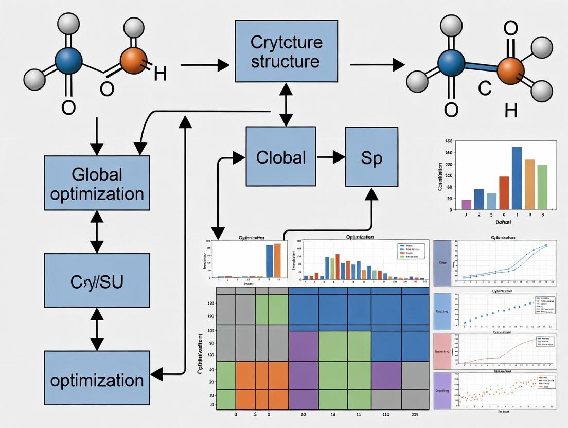
2. Core CSP Workflow and Methodology The following diagram illustrates the logical flow of a modern, computationally-driven CSP study, framed within a global optimization paradigm.
Title: Global Optimization Workflow for Crystal Structure Prediction
3. Step-by-Step Experimental Protocol
3.1 Step 1: Molecular Preparation and Conformational Sampling
- Objective: Generate a representative set of low-energy molecular conformations for the flexible API.
- Protocol:
- Obtain the 3D molecular structure (e.g., from CSD, PubChem, or quantum chemical optimization).
- Perform a conformational search using software like Confab (Open Babel) or OMEGA (OpenEye). Use a root-mean-square deviation (RMSD) threshold of 0.5 Å for uniqueness.
- Optimize each unique conformer using Density Functional Theory (DFT) with a basis set like 6-31G(d) and a functional like B3LYP-D3.
- Calculate the relative energy of each conformer. Select all conformers within a 5-10 kJ/mol window above the global minimum for subsequent packing.
3.2 Step 2: Crystal Structure Generation via Global Sampling
- Objective: Globally sample the crystallographic degrees of freedom (space groups, molecular position/orientation).
- Protocol:
- Select common chiral space groups relevant for organic molecules (e.g., P2₁2₁2₁, P2₁, C2, P1).
- Using a CSP engine (GRACE, RandomSpg, or MERCURY), generate thousands of initial crystal packing arrangements ("crystal seeds") for each selected conformer and space group. Use stochastic search algorithms (e.g., Monte Carlo, particle swarm) to vary molecular position, orientation, and unit cell parameters.
- Typically, generate 5,000-10,000 seeds per conformer/space group combination.
3.3 Step 3: Force Field-Based Lattice Energy Minimization and Clustering
- Objective: Refine and rank the generated seeds, then remove duplicates.
- Protocol:
- Minimize the lattice energy of all generated seeds using an anisotropic, reparametrized force field (e.g., W99, CE-B3LYP in DMACRYS or FFLUX). This step relaxes the structure to the nearest local minimum.
- Calculate the final lattice energy (E_FF) for each minimized structure.
- Perform cluster analysis on the minimized structures using unit cell parameters and molecular packing similarity (e.g., via Crystal Packing Similarity in MERCURY). Retain a single representative structure from each cluster (typically using an energy window of 2.5 kJ/mol and an RMSD threshold of 0.3 Å).
3.4 Step 4: High-Resolution Final Ranking with Density Functional Theory
- Objective: Accurately rank the relative stability of unique candidate structures.
- Protocol:
- Select the lowest-energy 50-100 unique structures from the force field stage.
- Perform full periodic DFT optimization using a van der Waals-inclusive functional (e.g., PBE-D3(BJ)) with a plane-wave basis set (e.g., in VASP or Quantum ESPRESSO). Use a kinetic energy cutoff of 500-600 eV and appropriate k-point spacing.
- Calculate the final lattice energy (E_DFT) and, if possible, the free energy (including thermal corrections via phonon calculations) for each fully optimized structure.
4. Data Analysis and Interpretation The final output is analyzed via an energy-rank plot, a critical tool for assessing prediction outcomes within the global optimization thesis.
Title: Energy-Rank Plot for Polymorph Stability Assessment
Table 1: Example CSP Output Data for a Hypothetical API
| Rank | Space Group | DFT Lattice Energy (kJ/mol) | Density (g/cm³) | Relative Energy vs. Global Min (kJ/mol) | Experimental Match? |
|---|---|---|---|---|---|
| 1 | P2₁2₁2₁ | -215.4 | 1.345 | 0.0 | Predicted (Form I) |
| 2 | P2₁ | -213.9 | 1.321 | 1.5 | Known (Form II) |
| 3 | P1 | -212.1 | 1.298 | 3.3 | Predicted |
| 4 | C2 | -210.5 | 1.310 | 4.9 | Known (Form III) |
| 5 | P2₁2₁2₁ | -208.7 | 1.285 | 6.7 | Predicted |
5. The Scientist's Toolkit: Essential Research Reagent Solutions
Table 2: Key Computational Tools and Resources for CSP
| Item/Software | Function in CSP Protocol | Key Application Note |
|---|---|---|
| GRACE (Global System) | Integrated CSP platform combining conformational search, packing generation, force field & DFT minimization. | End-to-end workflow automation. |
| DMACRYS | Lattice energy minimization software using accurate, anisotropic atom-atom force fields. | Critical for Stage 3 refinement and initial ranking. |
| VASP (Vienna Ab initio Simulation Package) | Periodic DFT code for high-resolution geometry optimization and energy calculation. | Used in Stage 4 for final ranking accuracy. |
| CSD (Cambridge Structural Database) | Repository of experimentally determined organic crystal structures. | Source of initial molecule geometry; validation of predictions. |
| MERCURY (CSD Software) | Visualization and analysis of crystal structures; includes packing similarity and module for in silico crystallization. | Clustering analysis (Stage 3) and visualization of results. |
| Reparametrized Force Field (e.g., W99) | A tailor-fit intermolecular potential for accurate description of non-covalent interactions. | Provides reliable initial energy landscape for global optimization sampling. |
Application Notes
The accurate prediction and characterization of multi-component crystalline forms—including solvates, hydrates, and cocrystals—is a critical frontier in crystal structure prediction (CSP). Within the thesis of Global optimization for crystal structure prediction research, these systems represent a stringent test for computational methodologies, demanding algorithms that can navigate complex, high-dimensional energy landscapes to locate all experimentally plausible polymorphs and stoichiometries.
Current Challenges & Research Focus:
- Combinatorial Complexity: The search space expands multiplicatively with each additional component, requiring efficient global optimization to sample potential packing motifs.
- Variable Stoichiometry: Predicting stable 1:1, 2:1, or even higher-order stoichiometries adds another layer to the optimization problem.
- Solvent Role & Displacement: Algorithms must differentiate between stable, crystalline solvates and mere solvent inclusion, and predict hydrate stability under varying relative humidity.
- Thermodynamic Ranking: The final CSP landscape must be accurately ranked by free energy, requiring precise modeling of component-component and component-environment interactions.
The integration of advanced computational sampling with targeted experimental validation is key to transforming CSP from a supportive tool to a predictive engine in pharmaceutical and materials development.
Table 1: Comparative Analysis of Multi-Component Crystal Types
| Crystal Type | Definition | Typical Stability Drivers | Key Characterization Techniques | Impact on Drug Development |
|---|---|---|---|---|
| Hydrate | Crystal incorporating water molecules in a definite stoichiometric ratio. | Hydrogen bonding networks, lattice energy compensation for water displacement. | TGA, DVS, XRPD, ssNMR. | Alters solubility, chemical stability, and bioavailability. Hydrate formation can occur during processing or storage. |
| Solvate | Crystal incorporating solvent molecules other than water. | Specific host-solvent interactions (e.g., H-bond, halogen bond). Solvent polarity and size. | TGA-DSC, XRPD, solution calorimetry. | Desolvation can lead to phase transformation, amorphization, or collapse. Critical for controlling final form. |
| Pharmaceutical Cocrystal | Multi-component crystal with API and a GRAS coformer bonded via non-covalent interactions. | Complementary hydrogen bond donors/acceptors, molecular shape fitting. | SCXRD, PXRD, FTIR, melting point analysis. | Can dramatically improve physicochemical properties (solubility, dissolution, stability) without altering covalent chemistry. |
| Salt | Ionic multi-component crystal comprising ionized API and counterion. | Proton transfer driven by ΔpKa (>2-3). Electrostatic forces. | pH-solubility analysis, SCXRD, IR. | The most common strategy to modify solubility, dissolution rate, and bioavailability. |
Table 2: Global Optimization Parameters for CSP of Multi-Component Systems
| Computational Parameter | Single-Component CSP | Two-Component (e.g., Cocrystal) CSP | Considerations for Solvates/Hydrates |
|---|---|---|---|
| Search Space Dimensions | Molecular position, orientation, conformation. | Adds variables for coformer relative position/orientation. | Adds solvent molecule degrees of freedom; potential for disorder modeling. |
| Typical Candidate Structures Generated | 1,000 - 100,000 | 10,000 - 1,000,000+ | Highly variable; depends on solvent site occupancy and symmetry. |
| Dominant Energy Terms | Van der Waals, conformational strain, electrostatic. | Adds specific intermolecular interactions (H-bonds, π-π). | Strong polarity and H-bonding of solvent; entropic contributions to free energy are significant. |
| Key Ranking Challenge | Accurate relative lattice energy differences (< 2 kJ/mol). | Modeling component-component interaction energy vs. pure component lattice energies. | Predicting solvent occupation stability vs. desolvated/apostructure. |
Experimental Protocols
Protocol 1: Slurry Conversion Experiment for Hydrate/Solvate Stability Screening Objective: To experimentally determine the most thermodynamically stable crystalline form (including solvates/hydrates) under specific solvent conditions. Materials: See "The Scientist's Toolkit" (Section 5). Procedure:
- Preparation: Place approximately 50-100 mg of the API (or a mixture of API and coformer for cocrystals) into 2 mL glass vials.
- Solvent Addition: To each vial, add 0.5 mL of a selected pure solvent or solvent/water mixture (e.g., water, methanol, ethanol, acetone, ethyl acetate).
- Slurrying: Cap the vials and place them on a temperature-controlled orbital shaker/rocker. Agitate at a constant temperature (e.g., 25°C) for a minimum of 7 days.
- Monitoring: Periodically check vials for any signs of dissolution or oiling out. After 7 days, sample the solid phase.
- Analysis: Filter the suspension using a vacuum filtration setup with a 0.45 µm filter. Quickly analyze the wet solid by XRPD. Allow a portion to air-dry, then re-analyze by XRPD and TGA to assess desolvation.
- Interpretation: The XRPD pattern of the wet solid indicates the stable form in equilibrium with that solvent. Drying patterns reveal the stability of the solvate/hydrate.
Protocol 2: Dynamic Vapor Sorption (DVS) for Hydrate Stability & Stoichiometry Objective: To quantify the hygroscopicity of a material and identify stable hydrate stoichiometries. Materials: DVS instrument, high-precision microbalance, sample pans, dry nitrogen gas. Procedure:
- Initialization: Pre-dry the DVS sample chamber with dry nitrogen. Accurately weigh (5-20 mg) of sample into a tared pan.
- Equilibration: Place the sample in the DVS and expose it to a dry nitrogen flow (0% RH) at constant temperature (e.g., 25°C) until the mass change (dm/dt) is less than 0.002% per minute for at least 10 minutes. Record this as the dry mass.
- Sorption Cycle: Program a stepwise isothermal protocol. Typically, increase RH in 10% increments from 0% to 90% RH, then decrease in the same steps back to 0% RH. At each step, hold until equilibrium (same dm/dt criterion as above).
- Data Collection: The instrument records mass vs. time and RH. Plot the equilibrium mass at each step against %RH to create sorption/desorption isotherms.
- Analysis: Sharp, reversible mass gains at specific RH points indicate the formation of a stable crystalline hydrate. The plateau mass corresponds to a specific stoichiometry (e.g., monohydrate, dihydrate). Hysteresis between sorption and desorption curves suggests kinetically trapped forms or phase transformations.
Diagrams
Title: CSP Workflow for Multi-Component Systems
Title: Experiment-Computation Feedback Loop
The Scientist's Toolkit
Table 3: Essential Research Reagent Solutions & Materials
| Item Name | Category | Function & Application |
|---|---|---|
| Polymorph Screening Kit | Consumable/Kit | Pre-portioned mixtures of common pharmaceutical solvents and polymers for high-throughput crystallization experiments. |
| Si-Microwave Well Plates | Laboratory Hardware | Low-background plates for high-throughput XRPD analysis of microcrystalline samples from screening. |
| DVS Intrinsic | Instrumentation | Measures minute mass changes due to water/solvent sorption; critical for characterizing hydrates, solvates, and amorphous content. |
| TGA-DSC 3+ | Instrumentation | Simultaneous thermal gravimetric and calorimetric analysis. Essential for determining solvate loss temperature, weight %, and associated enthalpy. |
| Cambridge Structural Database (CSD) | Software/Database | Repository of experimentally determined organic and metal-organic crystal structures. Used for interaction propensity analysis (H-bond, π-stacking) and force field validation. |
| GRACE Coformer Library | Chemical Library | A curated collection of Generally Regarded As Safe (GRAS) molecules for pharmaceutical cocrystal screening. |
| Anti-Solvent (Heptane, Cyclohexane) | Chemical Reagent | Used in crystallization experiments to reduce solubility and induce precipitation, often revealing metastable forms. |
| Perfluoroopolyether Oil | Laboratory Reagent | Used for mounting and protecting air-/moisture-sensitive crystals during single-crystal X-ray diffraction data collection. |
Overcoming Computational Hurdles: Troubleshooting CSP Workflows
Global optimization for crystal structure prediction (CSP) aims to locate the global minimum on the potential energy surface (PES), corresponding to the thermodynamically stable crystal structure. Convergence failures occur when optimization algorithms fail to locate any minimum efficiently, while false minima are local free energy minima mistaken for the global minimum. These pitfalls directly impact the reliability of in silico drug polymorph screening.
Quantitative Analysis of Common Pitfalls
Table 1: Prevalence and Impact of Pitfalls in CSP Studies (2019-2024)
| Pitfall Category | Reported Frequency (%) | Avg. CPU Time Cost (Core-Hours) | Impact on Predicted Lattice Energy (kJ/mol) | Key Contributing Factor |
|---|---|---|---|---|
| Convergence Failure (Sampling) | 35-45% | 12,000 - 18,000 | N/A (No result) | Incomplete configurational sampling |
| Convergence Failure (Relaxation) | 15-20% | 3,000 - 5,000 | N/A | Poor force field gradient accuracy |
| False Minima (Ranking Error) | 25-30% | All expended | 5 - 25 (vs. true global min) | Inadequate free energy model |
| False Minima (Symmetry Trapping) | 10-15% | Varies | 2 - 15 | Algorithmic symmetry bias |
Table 2: Algorithm Performance Against Pitfalls
| Optimization Method | Resilience to Convergence Failure | Resilience to False Minima | Typical CSP Application |
|---|---|---|---|
| Genetic Algorithms (GA) | Moderate-High | Moderate | Initial global search |
| Simulated Annealing (SA) | Moderate | Low-Moderate | Conformational space |
| Particle Swarm (PSO) | High | Moderate | Cluster hydrates |
| Basin Hopping | High | High | Lattice energy min. |
| Random Search | Low (inefficient) | Very Low | Benchmarking |
Experimental Protocols
Protocol 3.1: Systematic Sampling to Mitigate Convergence Failure
Objective: Ensure comprehensive exploration of the crystal packing hyperspace.
- Define Degrees of Freedom: For a molecule with Z'=1, define search variables: 3 lattice parameters (a, b, c), 3 angles (α, β, γ), 3 translational coordinates, and 3 rotational Euler angles.
- Initial Population Generation (for GA): Use a diversified seeding protocol.
- Generate 1000 random structures within physically plausible bounds (e.g., density 0.8-1.4*g/cm³).
- Apply space group symmetry operators (common: P1, P2₁, P2₁2₁2₁, C2/c, P2₁/c) to each candidate.
- Reject structures with unphysical intermolecular clashes (atomic overlap < 0.8 * sum of van der Waals radii).
- Parallel Evaluation: Distribute initial population across HPC nodes. For each candidate, perform a preliminary geometry optimization using a fast semi-empirical (PM7) or molecular mechanics (GAFF) method to quench high-energy strains.
- Iterative Evolution (GA Cycle):
- Selection: Retain top 30% lowest-energy structures. Apply a fitness-proportional selection for breeding.
- Crossover: For two parent structures, swap random lattice vectors or molecular orientation quaternions with 40% probability.
- Mutation: Randomly perturb a chosen variable (e.g., ±15° rotation, ±0.5 Å translation) with 20% probability. Introduce a new random structure with 5% probability to maintain diversity.
- Continue for 100 generations or until energy distribution plateau is observed.
Protocol 3.2: Free Energy Ranking to Discern False Minima
Objective: Accurately rank candidate structures using finite-temperature free energy.
- Post-Global Optimization Filtering: Take the 50 lowest lattice energy structures from Protocol 3.1.
- Lattice Dynamics (Quasi-Harmonic Approximation - QHA):
- For each candidate, perform full ab initio (e.g., PBE-D3) geometry optimization to a tight convergence threshold (forces < 0.001 eV/Å).
- Compute the harmonic phonon density of states on a 3x3x3 q-point grid.
- Calculate vibrational free energy (F_vib) at 298 K, integrating over the Brillouin zone.
- Explicit Free Energy Correction (Molecular Dynamics):
- For the top 10 candidates from QHA, construct a 3x3x3 supercell.
- Perform an NPT molecular dynamics simulation (300 K, 1 atm) using a validated force field (e.g., FIT). Length: 200 ps equilibration, 500 ps production.
- Use the production phase to calculate the ensemble average of enthalpy ⟨H⟩.
- Compute Gibbs Free Energy G = ⟨H⟩ - T*S, where entropy S is estimated via the Two-Phase Thermodynamics (2PT) method applied to the velocity autocorrelation function.
- Final Ranking: Rank candidates by the computed Gibbs Free Energy at ambient conditions.
Visualizations
Diagram 1: CSP Optimization Workflow & Pitfalls
Diagram 2: Free Energy Ranking Protocol
The Scientist's Toolkit: Research Reagent Solutions
Table 3: Essential Computational Tools for Robust CSP
| Tool/Reagent Category | Specific Example(s) | Function & Rationale |
|---|---|---|
| Global Search Software | GAtor, GRACE, RandomSearch | Provides algorithms for comprehensive exploration of crystal energy landscapes, mitigating initial convergence failure. |
| Force Fields (FF) | FIT (Polymorphic), GAFF, custom-tailored FF | Enable rapid energy/force evaluations during sampling. Accuracy is critical to avoid false minima. |
| Ab Initio Electronic Structure | VASP (PBE-D3), Quantum ESPRESSO, CRYSTAL | Deliver high-accuracy lattice energies and phonon spectra for final ranking and QHA. |
| Free Energy Computation | Phonopy (QHA), LAMMPS/MD+2PT code, Shake-the-Box | Calculate temperature-dependent free energy corrections to correctly rank polymorph stability. |
| Structure Analysis & Clustering | XtalComp, Pymatgen, CCDC Tools | Identify and remove duplicate structures, analyze packing motifs, and detect symmetry trapping. |
| High-Performance Computing (HPC) Environment | Slurm/PBS job schedulers, MPI/OpenMP parallelized codes | Enables the computationally intensive sampling and high-level calculations required for reliable CSP. |
Within the framework of global optimization for crystal structure prediction (CSP), evolutionary and genetic algorithms (GAs) are pivotal for navigating complex, high-dimensional energy landscapes. The efficacy of these algorithms is critically dependent on the careful tuning of search parameters, namely population size (N), mutation rate (μ), and stopping criteria. This document provides detailed application notes and experimental protocols for optimizing these parameters to enhance the reliability and efficiency of CSP in materials science and pharmaceutical development.
Quantitative Parameter Benchmarks for CSP
The following table synthesizes current recommendations from literature and practice for GA parameters in CSP using common software (e.g., USPEX, GAtor, CALYPSO).
Table 1: Recommended Ranges for Key GA Parameters in CSP
| Parameter | Typical Range | Impact on Search | Recommended Starting Point for CSP |
|---|---|---|---|
| Population Size (N) | 10 - 100 structures per generation | Small N: Faster but risk of premature convergence. Large N: Better sampling but higher computational cost. | 20-30 for systems with <10 atoms; 30-60 for larger/more complex systems. |
| Mutation Rate (μ) | 0.1 - 0.5 per structure (10%-50%) | Low μ: Exploitation, risk of stagnation. High μ: Exploration, may disrupt good solutions. | 0.3 (30% of offspring undergo mutation). |
| Crossover Rate | 0.6 - 0.9 per structure (60%-90%) | Primary driver for combining structural motifs. | 0.7 (70% of offspring from crossover). |
| Stopping Generation | 20 - 100 generations | Fixed budget; must be balanced with N for total cost. | Monitor convergence; stop when best fitness unchanged for 20-30 generations. |
| Energy Convergence Threshold (ΔE) | 10⁻³ - 10⁻⁵ eV/atom | Defines stability of found minima. | Stop when global minimum candidate's energy change < 0.001 eV/atom over 10 generations. |
Experimental Protocols for Parameter Optimization
Protocol 3.1: Systematic Calibration of Population Size and Mutation Rate
Objective: To empirically determine the optimal (N, μ) pair for a given CSP problem class (e.g., organic molecular crystals). Materials: As per "Scientist's Toolkit" below. Procedure:
- Define Test Set: Select 2-3 known benchmark crystal systems with established global minimum structures.
- Design Experiment: Create a grid of parameters: N = [20, 40, 60] and μ = [0.1, 0.3, 0.5]. Keep crossover rate constant at 0.7.
- Run Iterations: For each (N, μ) pair, execute the GA for 50 generations. Perform 5 independent runs to account for stochasticity.
- Data Collection: Record for each run:
- Success Rate (SR): Fraction of runs locating the global minimum.
- Mean Best Energy vs. Generation.
- Total Computational Cost (CPU-hours).
- Analysis: Plot SR and cost versus parameter pairs. The optimal region maximizes SR while minimizing cost.
Protocol 3.2: Establishing Adaptive Stopping Criteria
Objective: To implement a robust, problem-agnostic stopping rule. Procedure:
- Monitor Key Metrics: Track per generation: a) Best enthalpy, b) Average enthalpy of population, c) Diversity metric (e.g., average RMSD between structures).
- Set Convergence Conditions: Stop the search when ALL of the following are met for a user-defined window (e.g., 25 generations):
- Energy Plateau: Δ(Best Enthalpy) < threshold (e.g., 0.005 eV/atom).
- Population Stability: Δ(Average Enthalpy) < threshold.
- Diversity Loss: Population diversity drops below 15% of initial diversity.
- Fallback Criterion: Implement a hard upper limit on total number of energy evaluations (e.g., 50,000) as a safety net.
Visualizations
Title: Genetic Algorithm Workflow for Crystal Structure Prediction
Title: Parameter Optimization and Calibration Protocol
The Scientist's Toolkit: Research Reagent Solutions
Table 2: Essential Materials & Computational Tools for CSP Parameter Optimization
| Item | Function & Explanation |
|---|---|
| CSP Software (USPEX/GAtor) | Core platform implementing the genetic algorithm for searching crystal energy landscapes. |
| DFT Code (VASP, Quantum ESPRESSO) | First-principles calculator used for accurate enthalpy (fitness) evaluation of candidate structures. |
| High-Performance Computing (HPC) Cluster | Essential for parallel execution of multiple energy calculations and independent GA runs. |
| Reference Benchmark Structures | Known crystal structures (from CSD, ICDD) used to validate search success rates and parameter efficacy. |
| Structure Analysis Scripts (Python) | Custom scripts to compute metrics like diversity (RMSD), track convergence, and analyze results. |
| Interatomic Potentials (FF/ML) | Approximate, fast potentials for initial screening or systems where DFT is prohibitively expensive. |
In crystal structure prediction (CSP) and materials discovery, global optimization algorithms search the vast, high-dimensional potential energy surface (PES) for the most stable atomic configurations. The fidelity, speed, and cost of this search are fundamentally governed by the energy model employed. The choice between classical Force Fields (FF), quantum-mechanical Density Functional Theory (DFT), and Machine Learning (ML) potentials represents a critical trade-off between computational accuracy and resource expenditure. This application note, framed within a thesis on global optimization for CSP, provides a structured comparison and detailed protocols to guide researchers and drug development professionals in selecting and deploying the appropriate model for their specific research phase.
Quantitative Comparison of Energy Models
The table below summarizes the key quantitative metrics for the three primary energy model classes, based on current benchmarks (2023-2024).
Table 1: Comparative Analysis of Energy Models for CSP
| Feature | Classical Force Fields (FF) | Density Functional Theory (DFT) | Machine Learning Potentials (ML) |
|---|---|---|---|
| Computational Cost | ~10⁻⁶ to 10⁻³ CPU-hr/atom | ~1 to 10² CPU-hr/atom | ~10⁻⁴ to 10⁻² CPU-hr/atom (Inference) |
| Typical System Size | 10⁴ – 10⁸ atoms | 10 – 10³ atoms | 10² – 10⁶ atoms |
| Accuracy (vs. Exp.) | Low to Moderate (FF-dependent) | High (Chemical accuracy possible) | Near-DFT (when trained well) |
| Physics Basis | Parametric classical potentials | Quantum mechanics (electron density) | Data-driven interpolation |
| Training Data Cost | N/A (Parameter fitting) | N/A (Reference method) | High (Requires 10³–10⁵ DFT frames) |
| Transferability | System-specific, poor for new chemistries | Universally applicable | Limited to training domain |
| Key Limitation | Cannot describe bond breaking/forming | Scaling with electrons, functional choice | Data hunger, extrapolation risk |
| Best Use Case in CSP | Pre-screening, large-scale dynamics, polymers | Final validation, electronic properties, small units | High-accuracy screening of configurational space |
Experimental Protocols for Model Deployment in CSP Workflows
Protocol 3.1: Multi-Stage Screening Using a FF → ML → DFT Cascade
Objective: To efficiently identify low-energy crystal polymorphs of an organic drug molecule while balancing computational cost.
Materials & Software: Open Babel (preprocessing), GROMACS or LAMMPS (FF), SCHNATPACK or MACE (ML), VASP or CP2K (DFT), Global optimization toolkit (e.g., GAtor, AIRSS).
Procedure:
- Conformer Generation: Generate an ensemble of 100-1000 reasonable molecular conformers using a tool like RDKit or CREST.
- FF-Based Packing: Use a classical force field (e.g., GAFF, OPLS-AA) within a crystal packing algorithm (e.g., in GROMACS) to generate thousands of initial crystal structures in common space groups.
- FF Relaxation & Ranking: Locally relax all structures with the same FF and rank them by lattice energy. Select the top 100-500 structures.
- ML Refinement: Re-evaluate and relax the selected subset using a high-quality ML potential (e.g., a model trained on organic molecules like ANI-2x, or a custom model). Re-rank based on ML-predicted energy.
- DFT Final Validation: Perform full DFT relaxation (using a functional like PBE-D3(BJ) or r²SCAN-DFT) on the top 20-50 ML-ranked structures. Calculate precise relative stabilities and electronic properties.
- Analysis: Compare predicted stable polymorphs with experimental data, analyzing the energy landscape.
Protocol 3.2: Active Learning for On-the-Fly ML Potential Development
Objective: To build a system-specific ML potential for a novel inorganic perovskite during a global structural search.
Materials & Software: ASE (Atomistic Simulation Environment), ML potential framework (MACE, Allegro), DFT code, active learning loop script.
Procedure:
- Initial Dataset Creation: Perform ab initio molecular dynamics (AIMD) on a few candidate perovskite structures (e.g., cubic, tetragonal phases) using DFT to generate ~100 training configurations.
- ML Model Training: Train an equivariant graph neural network potential (e.g., MACE) on this initial dataset.
- Active Learning Loop: a. Exploration: Use the current ML potential to drive a global optimization search (e.g., via particle swarm optimization) to propose new low-energy candidate structures. b. Uncertainty Quantification: For each proposed structure, compute the model's predictive uncertainty (e.g., using committee models or latent distance metrics). c. Selection & Query: Select the 10-20 candidates with the highest uncertainty or lowest predicted energy. d. DFT Calculation: Perform single-point DFT calculations on the selected candidates. e. Dataset Augmentation: Add these new (structure, DFT energy/forces) pairs to the training dataset. f. Model Retraining: Re-train the ML potential on the augmented dataset.
- Convergence: Repeat Step 3 until no new, stable structures are found, and the model's predictions on new candidates converge (uncertainty falls below a threshold).
- Final Search: Execute an extensive global optimization run using the final, robust ML potential to map the PES.
Visualizing the Decision and Workflow Logic
Title: Decision Tree for Energy Model Selection in CSP
Title: Three-Stage CSP Workflow: FF to ML to DFT
The Scientist's Toolkit: Essential Research Reagent Solutions
Table 2: Key Software & Computational Resources for Energy Model Deployment
| Item | Function in CSP | Example/Provider |
|---|---|---|
| Global Optimization Software | Drives the structural search across the PES. | GAtor (Genetic Algorithm), AIRSS (Ab Initio Random Structure Search), CALYPSO (Particle Swarm). |
| Force Field Suites | Provides parameterized classical potentials for rapid energy/force calculations. | OpenMM, GROMACS, LAMMPS; Force fields: GAFF (organic), ReaxFF (reactive). |
| DFT Software Packages | Serves as the reference "gold standard" for accuracy and for generating ML training data. | VASP, Quantum ESPRESSO, CP2K, CASTEP. |
| ML Potential Frameworks | Enables training and deployment of high-speed, high-accuracy surrogate models. | MACE, Allegro, NequIP (E(3)-equivariant); SCHNATPack (SchNet). |
| Automation & Workflow Tools | Manages complex, multi-step simulation protocols and data pipelines. | ASE (Atomic Simulation Environment), FireWorks, signac. |
| Active Learning Managers | Orchestrates the iterative data generation and model training loop. | FLARE, AL4ED, custom scripts using ASE and ML framework APIs. |
| High-Performance Computing (HPC) | Essential infrastructure for DFT calculations and large-scale ML training/inference. | CPU/GPU clusters (e.g., Slurm-managed), Cloud computing (AWS, GCP, Azure). |
Dealing with Disordered and Flexible Molecules
Within the global optimization framework for crystal structure prediction (CSP), the treatment of disordered and conformationally flexible molecules represents a significant frontier. The inherent complexity of these systems, characterized by multiple low-energy conformations and positional disorder, challenges traditional CSP methodologies that often assume rigid molecular models. Successfully predicting stable crystal forms for such molecules, particularly active pharmaceutical ingredients (APIs), is critical for drug development, impacting solubility, bioavailability, and intellectual property. This application note details protocols and strategies for integrating disorder and flexibility into global CSP workflows.
Theoretical Framework and Challenges
The potential energy surface (PES) for flexible molecules is highly multimodal. The global minimum on the isolated molecule's conformational landscape may not correspond to the molecular conformation present in the global minimum of the crystal lattice energy landscape. This necessitates a coupled optimization of conformational and crystallographic degrees of freedom. Key quantitative challenges include:
- Conformational Sampling: The number of plausible rotatable bonds exponentially increases the conformational space.
- Lattice Energy Evaluation: Accurate relative energies between polymorphs require highly sensitive modeling of weak intermolecular forces, which can be conformation-dependent.
- Entropy Contribution: At finite temperatures, entropic contributions from molecular vibrations and disorder can stabilize certain phases.
Table 1: Energy Scales in CSP for Flexible Molecules
| Energy Component | Typical Magnitude (kJ/mol) | Challenge for Flexible Molecules |
|---|---|---|
| Conformational Barrier | 5 - 50 | Defines number of distinct conformers to sample. |
| Intermolecular Lattice Energy | 50 - 150 | Sensitive to small conformational changes. |
| Polymorph Energy Difference | 0.1 - 5 | Often less than conformational energy penalties. |
| Vibrational/Entropic Contribution (TΔS) | 0 - 10 | Can reverse stability ranking based solely on lattice energy. |
Core Protocols
Protocol 1: Conformer Generation and Pre-screening
Objective: Generate a representative, low-energy set of molecular conformations for input into CSP calculations.
Methodology:
- Initial Sampling: Use a stochastic method (e.g., Monte Carlo) or systematic torsional grid search (e.g., 60° increments) around all rotatable bonds. Software: OMEGA, CONFLEX, or RDKit.
- Geometry Optimization: Optimize all generated structures using a force field (e.g., GAFF2, MMFF94s) or semi-empirical quantum mechanics (e.g., GFN2-xTB) to remove strain.
- Clustering and Ranking: Cluster optimized conformers based on root-mean-square deviation (RMSD) of atomic positions (typical cutoff: 0.5 Å). Select the lowest-energy representative from each cluster.
- Quantum Mechanical Refinement: Further optimize and calculate accurate relative energies for the top-ranked conformers (e.g., 20-50) using Density Functional Theory (DFT) with a dispersion-corrected functional (e.g., ωB97X-D/def2-SVP).
- Boltzmann Population Analysis: Calculate the relative population of each conformer at room temperature (298 K) based on the DFT electronic energies and quasi-harmonic vibrational free energy corrections.
Critical Parameters: Choice of force field, energy window for saving conformers (e.g., 50 kJ/mol from global minimum), clustering algorithm sensitivity, and DFT functional selection.
Protocol 2: CSP with Explicit Flexibility (Multi-Conformer CSP)
Objective: Perform a global crystal structure search using multiple molecular conformations simultaneously.
Methodology:
- Input Preparation: Prepare a set of pre-optimized, distinct molecular conformers from Protocol 1. Common practice is to use conformers within 10-15 kJ/mol of the global minimum.
- Global Lattice Energy Minimization: Use a CSP engine (e.g., CrystalPredictor, GRACE, RandomSearch) that treats molecular conformation as a variable. The search operates in a combined space of crystal packing variables (unit cell parameters, molecular position/orientation) and selected torsional angles.
- Clustering and Ranking of Crystal Structures: After the search, cluster resulting crystal structures based on packing similarity. For each cluster, select the lowest-energy structure.
- High-Level Lattice Energy Minimization: Re-minimize the lattice energy of the top-ranked, unique crystal structures using a more accurate model (e.g., tailored force fields or DFT-D).
- Free Energy Ranking: Estimate the relative thermodynamic stability of predicted polymorphs by calculating the Gibbs free energy, incorporating phonon contributions from lattice dynamics calculations.
Table 2: Comparison of CSP Strategies for Flexible Molecules
| Strategy | Description | Advantage | Disadvantage |
|---|---|---|---|
| Rigid Molecule | Use single, lowest-energy gas-phase conformer. | Computationally cheap, simple. | Misses conformer-specific packing motifs. |
| Multi-Conformer | Perform separate CSP runs for each fixed conformer. | Captures conformer-specific packing. | Misses coupling between conformation and packing. |
| Explicit Flexibility | Treat conformation as variable during CSP search. | Most comprehensive, allows coupling. | Highly computationally expensive, larger search space. |
Workflow for CSP of Flexible Molecules
Protocol 3: Modeling Disordered Solvates and Ionic Complexes
Objective: Predict stable crystalline forms for systems with compositional or positional disorder, such as hydrates, solvates, or salt co-formers.
Methodology:
- Stoichiometry Variation: For solvates, perform separate CSP searches for likely stoichiometries (e.g., anhydrate, monohydrate, dihydrate).
- Site Disorder Simulation: For systems where a molecule or ion can occupy multiple positions, use CSP to generate structures with the component in different plausible orientations/locations.
- Energy vs. Composition Plotting: Calculate the lattice energy per API molecule for each predicted structure. Plot energy against solvent/salt content.
- Assessment of Stability: The most thermodynamically stable form under given conditions is determined by the minimum of the energy-composition curve, often considering the chemical potential of the disordered component (e.g., water vapor pressure).
The Scientist's Toolkit
Table 3: Key Research Reagent Solutions for CSP of Flexible Molecules
| Item / Software | Primary Function | Key Consideration |
|---|---|---|
| Conformer Generator(e.g., OMEGA, RDKit, CONFLEX) | Samples the molecule's intrinsic conformational space. | Balance between exhaustiveness and computational cost. Torsional libraries and rules. |
| Quantum Chemistry Package(e.g., Gaussian, ORCA, psi4) | Provides accurate relative conformer energies and electrostatic potentials. | Choice of functional and basis set critical for weak interactions (DFT-D3/D4). |
| CSP Software with Flexibility(e.g., GRACE, CrystalPredictor II, MOF) | Performs global optimization over packing and conformational variables. | Efficiency of search algorithm in high-dimensional space. |
| Lattice Dynamics Code(e.g., PHONOPY, DMACRYS) | Calculates vibrational free energy contributions to stability. | Treatment of anharmonicity is challenging but important. |
| Tailored Force Field(e.g., FIT, Williams' Models) | Provides fast, accurate lattice energy evaluation during CSP search. | Parameterization must be robust for diverse packing motifs. |
Core Trade-offs in Flexible Molecule CSP
Integrating molecular flexibility and disorder into global CSP optimization is no longer optional for predictive accuracy in pharmaceutical and materials research. The protocols outlined advocate for a hierarchical approach: rigorous conformer generation, followed by a CSP strategy (multi-conformer or explicitly flexible) chosen based on molecular complexity and computational resources. The ultimate goal is a workflow that reliably produces a ranked list of thermodynamically plausible crystal structures, where the experimentally observed forms—including those with disorder—are found among the low-energy predictions. This capability is fundamental to de-risking solid-form selection in drug development.
Strategies for Reducing Dimensionality and Pre-screening Candidate Spaces
Within global optimization for crystal structure prediction (CSP), the search space for stable polymorphs is astronomically large. The central challenge is efficiently navigating this high-dimensional energy landscape to identify low-energy structures without exhaustive sampling. This document outlines application notes and protocols for dimensionality reduction and pre-screening strategies critical to modern CSP workflows, enabling feasible drug polymorph discovery.
Dimensionality Reduction Strategies
Reducing the number of degrees of freedom simplifies the energy landscape.
Symmetry and Space Group Restriction
Early-stage search is often constrained to common space groups. Data from the Cambridge Structural Database (CSD) indicates the prevalence of specific space groups for organic molecules.
Table 1: Prevalence of Common Space Groups in Organic CSP (CSD Data)
| Space Group | Frequency in Organic Crystals (%) | Typical Degrees of Freedom Reduction |
|---|---|---|
| P2₁/c | ~35% | ~55-70% |
| P-1 | ~20% | ~40-60% |
| P2₁2₁2₁ | ~10% | ~50-65% |
| C2/c | ~5% | ~60-75% |
Protocol 1.1: Symmetry-Constrained Search Setup
- Input: Molecular connectivity (e.g., SMILES, .mol file).
- Generate Z-matrices: Define internal coordinates (bond lengths, angles, torsion angles) for the asymmetric unit.
- Select Target Space Groups: Choose a subset (e.g., top 4 from Table 1) based on molecular symmetry and CSD statistics.
- Apply Symmetry Operations: Use crystallographic software (e.g.,
pymatgen,ASE) to generate full unit cells from the asymmetric unit using the symmetry operations of each selected space group. - Initialize Variables: For global optimization, define variables typically as (a) lattice parameters (angles constrained by space group), (b) molecular position/orientation within asymmetric unit, (c) key torsion angles.
Collective Variable (CV) Selection
Instead of optimizing all atomic coordinates, dynamics are projected onto key collective variables.
Protocol 1.2: Identifying Collective Variables for Molecular Crystals
- Conformational Analysis: Perform a relaxed rotational scan for all flexible torsion angles in the isolated molecule using DFT (B3LYP/6-31G*).
- Identify Low-Energy Torsions: Select torsion angles with energy barriers < ~5 kcal/mol as soft variables; fix others at their global minima.
- Intermolecular CVs: For known dimer or chain motifs (from CSD analogues), define CVs such as:
- Center-of-mass distances between specific molecular pairs.
- Slip-stack displacement angles.
- Hydrogen-bond lengths and angles.
- Embed in Optimizer: Use these CVs as the primary search dimensions in a Monte Carlo or genetic algorithm, with local relaxations permitted in full coordinate space.
Title: Workflow for Collective Variable Identification
Pre-screening Candidate Spaces
Rapid elimination of high-energy regions prior to expensive DFT calculations.
Hierarchical Filtering with Empirical Force Fields
A multi-stage filtering approach using increasingly accurate, but costly, methods.
Table 2: Hierarchical Pre-screening Protocol Performance
| Filter Stage | Method/Force Field | Avg. Time per Structure | Typical Rejection Rate | Key Function |
|---|---|---|---|---|
| Initial Generation | Random/GA in reduced CV | < 1 sec | N/A | Broad sampling |
| Stage 1 Filter | UFF or MMFF94 | 1-5 sec | ~70% | Remove steric clashes, very high energy |
| Stage 2 Filter | Repulsive-only (e.g., W99) | ~2 sec | ~50% of remainder | Refine packing, weak vdW |
| Stage 3 Filter | DFTB or xTB | 10-60 sec | ~40% of remainder | Approximate electronics, polarization |
| Final Ranking | DFT (PBE-D3) | Minutes to hours | N/A | Accurate energy ranking |
Protocol 2.1: Automated Hierarchical Filtering Workflow
- Stage 0 - Sampling: Generate 50,000-100,000 candidate crystal structures using a genetic algorithm operating in the reduced CV space (from Protocol 1.2).
- Stage 1 - Steric Clash Filter: Minimize all candidates using Universal Force Field (UFF) with a steepest-descent algorithm (max 100 steps). Discard any structure where minimization fails or energy is above a threshold (e.g., 100 kJ/mol above the lowest observed UFF energy).
- Stage 2 - Packing Filter: Minimize survivors using a repulsion-dispersion force field (e.g., Williams' W99 potential). Discard structures using energy/volume criteria.
- Stage 3 - Semi-empirical Filter: Perform a single-point energy calculation using GFN-xTB for all remaining candidates (~5,000-10,000). Cluster structures by energy and similarity (RMSD < 0.5 Å). Select the 100-200 lowest-energy unique representatives.
- Output: Pass the final shortlist to periodic DFT for relaxation and final energy ranking.
Title: Hierarchical Pre-screening Funnel
Machine Learning-Based Surrogate Models
Train a regressor to predict approximate lattice energies directly from a structural descriptor, bypassing early force field calculations.
Protocol 2.2: Implementing a ML Surrogate Filter
- Create Training Set: For the target molecule, generate 10,000 random crystal structures. Calculate their accurate lattice energy using a mid-tier method (e.g., DFTB).
- Featurization: Encode each crystal structure into a fixed-length vector using the Smooth Overlap of Atomic Positions (SOAP) descriptor (radius ~5 Å,
l_max=8,n_max=6). - Model Training: Train a Kernel Ridge Regression (KRR) or a Gradient Boosting model (e.g., XGBoost) on 8,000 structures to map SOAP vectors to DFTB energies.
- Validation: Tune hyperparameters on a 1,000-structure validation set. Target mean absolute error (MAE) < 3-5 kJ/mol.
- Deployment for Screening: For new candidate structures (e.g., from a GA), compute the SOAP descriptor and predict energy via the ML model. Reject all structures predicted to be > 25 kJ/mol above the current best prediction.
The Scientist's Toolkit: Research Reagent Solutions
Table 3: Essential Software and Computational Tools for CSP Pre-screening
| Item (Software/Package) | Category | Primary Function in Pre-screening |
|---|---|---|
| GRACE / PyXtal | Structure Generation | Generates random crystal structures within symmetry constraints for initial sampling. |
| RDKit | Cheminformatics | Handles molecular manipulation, conformational analysis, and Z-matrix generation. |
| Python Materials Genomics (pymatgen) | Crystal Analysis | Applies symmetry operations, analyzes structures, and computes structural descriptors. |
| Universal Force Field (UFF) | Empirical FF | Provides rapid, generic energy evaluation for Stage 1 steric filtering. |
| GFN-xTB | Semi-empirical QM | Delivers fast quantum-mechanical energy approximations for Stage 3 filtering. |
| DScribe / QUIP | Descriptor Tools | Calculates SOAP and other atomic descriptors for ML surrogate models. |
| Gaussian / ORCA | Quantum Chemistry | Performs conformational scans and final DFT energy evaluations (benchmarking). |
| CALYPSO / USPEX | Global Optimization | Implements evolutionary algorithms for searching reduced variable spaces. |
High-Performance Computing (HPC) Considerations for Large-Scale Searches
Thesis Context: This document provides application notes for leveraging High-Performance Computing (HPC) resources to accelerate large-scale configurational searches within global optimization workflows for crystal structure prediction (CSP). Effective HPC utilization is critical for exploring the vast, complex energy landscapes of molecular crystals to identify stable polymorphs, a cornerstone of computational solid-state chemistry and pharmaceutical development.
HPC Architecture Selection and Performance Metrics
The choice of HPC architecture dictates the parallelization strategy and scalability of CSP searches. Key quantitative performance data for current architectures is summarized below.
Table 1: Comparison of HPC Architectures for CSP Global Optimization Searges
| Architecture Type | Key Component | Typical Node Count (Range) | Memory/Node (GB) | Interconnect Bandwidth | Best Suited CSP Search Phase |
|---|---|---|---|---|---|
| CPU Cluster (Homogeneous) | Multi-core CPUs (e.g., AMD EPYC, Intel Xeon) | 10 - 100,000+ | 128 - 1024+ | 25 - 200 Gb/s (InfiniBand) | Energy minimization, Lattice dynamics, Data analysis |
| GPU-Accelerated Cluster | CPUs + NVIDIA/AMD GPUs (e.g., H100, MI250X) | 1 - 1000+ | 512 - 2048+ | 200 - 400 Gb/s (NVLink/InfiniBand) | High-throughput DFT (VASP, Quantum ESPRESSO), Neural network potentials |
| Cloud HPC (Elastic) | Virtualized CPUs/GPUs (AWS, Azure, GCP) | Scalable on-demand | Configurable (16-976 GB) | 10 - 100 Gb/s (Elastic Fabric Adapter) | Burst capacity for parallel candidate screening, Hybrid workflows |
Parallelization Strategies for Global Optimization
Effective parallelization is non-trivial for population-based global optimization algorithms (e.g., Genetic Algorithms, Particle Swarm Optimization) used in CSP.
Protocol 2.1: Coarse-Grained Parallelization for a Genetic Algorithm (GA) Search
- Objective: To parallelize the evaluation of fitness (energy) for a population of crystal structure candidates.
- Method:
- Master Process: Initializes a population of N candidate structures using random symmetric space groups and molecular orientations.
- Population Partitioning: The master process partitions the population into sub-populations equal to the number of available worker processes (P).
- Job Distribution: Each candidate structure is packaged with necessary computational parameters (DFT functional, basis set, k-point grid) and sent to a unique worker process via Message Passing Interface (MPI).
- Parallel Energy Calculation: Each worker process runs an independent electronic structure calculation (e.g., via CASTEP or Gaussian) on its assigned candidate(s).
- Result Aggregation: Workers return the computed total energy and stress tensor to the master process.
- Synchronization & Evolution: The master process applies GA operators (selection, crossover, mutation) to generate a new population, and the cycle repeats from step 2.
- HPC Considerations: This "embarrassingly parallel" approach scales well with the number of workers. The limiting factor is the load balancing, as individual energy calculations may have varying convergence times.
Title: Parallel Genetic Algorithm Workflow for CSP
Workflow Management and Data Handling
Large-scale searches generate petabytes of intermediate data. A robust workflow is essential.
Protocol 3.1: Implementing a Fault-Tolerant CSP Workflow using SLURM and Dask
- Objective: To manage a multi-stage CSP pipeline (generation → relaxation → ranking) with checkpointing and automatic job resubmission.
- Method:
- Workflow Definition: Define stages as separate Python scripts or executables (e.g.,
gen_candidates.py,relax_structures.py,rank_energies.py). - Dask Cluster Setup: Initialize a Dask cluster on the HPC job scheduler (SLURM/PBS). The Dask scheduler will manage task dependencies.
- Task Submission: Submit each candidate's relaxation as a delayed Dask task. Dask maps these tasks to the allocated worker nodes.
- Checkpointing: After each successful relaxation, the resulting structure and energy are written to a persistent, versioned database (e.g., MongoDB) or a filesystem with a unique hash (e.g., using
ase.db). - Fault Tolerance: If a worker node fails, Dask resubmits its assigned tasks to other available workers. The database checkpoint prevents redundant calculations.
- Result Collection: The final ranking task queries the database for all completed relaxations and sorts by lattice energy.
- Workflow Definition: Define stages as separate Python scripts or executables (e.g.,
Title: Fault-Tolerant CSP Pipeline with Dask and Database
The Scientist's Toolkit: Research Reagent Solutions
Table 2: Essential Software and Computational Resources for HPC-Enabled CSP
| Item Name | Category | Primary Function in CSP Search |
|---|---|---|
| AIRSS (Ab Initio Random Structure Searching) | Software Package | Generates random sensible crystal structures with symmetry constraints for initial population. |
| CALYPSO | Software Package | Performs particle swarm optimization-based structure prediction using evolutionary algorithms. |
| XtalOpt | Software Package | Open-source evolutionary algorithm for CSP, integrates with various DFT codes. |
| ASE (Atomic Simulation Environment) | Python Library | Provides tools for manipulating atoms, running calculations, and workflow scripting. |
| Dask & Joblib | Python Libraries | Enable parallel computing and workflow management on HPC clusters. |
| MPI (OpenMPI, MPICH) | Communication Protocol | Facilitates message passing between nodes for coarse-grained parallelization. |
| SLURM / PBS Pro | Job Scheduler | Manages resource allocation and job queuing on shared HPC systems. |
| Singularity / Apptainer | Containerization | Packages complex software stacks (DFT codes + dependencies) for portable, reproducible runs. |
| ParaDRAM | MCMC Sampler | Enables high-performance parallel Markov Chain Monte Carlo sampling of phase space. |
| Neural Network Potentials (e.g., MACE, NequIP) | Machine Learning Model | Provides quantum-accurate energy/force predictions at speeds ~10^6x faster than DFT for preliminary screening. |
Benchmarking Success: Validating and Comparing CSP Methodologies
The Cambridge Crystallographic Data Centre (CCDC) Blind Tests for crystal structure prediction (CSP) serve as the definitive, community-wide validation framework. Within the thesis context of Global optimization for crystal structure prediction research, these blind tests provide the critical experimental benchmark against which all optimization algorithms—whether based on genetic algorithms, simulated annealing, basin-hopping, or random search—must be rigorously evaluated. They transition CSP from a theoretical exercise to a validated predictive science by posing the core challenge: can a computational method correctly predict the experimentally observed crystal structure(s) of a given molecule from its chemical diagram alone, prior to synthesis?
The CCDC Blind Tests are periodic challenges that began in 1999. Each test provides participants with the 2D molecular diagrams of several organic molecules whose 3D crystal structures have been determined but not yet published. Participants submit up to three predicted crystal structures per molecule, ranked by likelihood. Success is measured by the ability to predict the experimental structure within a small threshold of geometric similarity (typically an RMSD of X Å for non-hydrogen atoms).
Table 1: Summary of CCDC Blind Test Results (I-IX)
| Blind Test | Year | No. of Target Molecules | Key Challenges Introduced | Success Rate (Top 3 Submissions) | Implications for Global Optimization |
|---|---|---|---|---|---|
| I | 1999 | 3 | Simple, rigid molecules. | Low | Established baseline; highlighted need for better search algorithms. |
| II | 2001 | 4 | Increased flexibility. | Moderate | Showed importance of conformational flexibility in search space. |
| III | 2004 | 4 | A salt, a hydrate. | Mixed | Necessitated inclusion of complex stoichiometry and proton transfer. |
| IV | 2007 | 4 | A co-crystal, larger molecules. | Improved | Demanded search over multi-component crystal landscapes. |
| V | 2010 | 5 | API-like molecules, polymorphism. | Higher | Forced methods to find multiple low-energy polymorphs. |
| VI | 2015 | 4 | Complex APIs with multiple torsions. | Significant | Validated advances in hierarchical search and lattice energy models. |
| VII | 2016 | 4 | Hydrates, salt, large flexible molecule. | Robust | Tested reliability on pharmaceutically relevant systems. |
| VIII | 2020 | 4 | Flexible macrocycle, salt, hydrate. | High | Demonstrated maturity of methods on "difficult" targets. |
| IX | 2023 | 4 | Complex functional groups, non-covalent motifs. | To be fully assessed | Ongoing test of current state-of-the-art. |
Note: Success rates are approximate and aggregate across all targets. Specific data should be sourced from the latest CCDC publications.
Experimental Protocols for Participation
The following protocol outlines the standard methodology for participating in a CCDC Blind Test, representing the de facto workflow for rigorous CSP validation.
Protocol: CCDC Blind Test Participation and Validation Workflow
A. Pre-Calculation Phase
- Registration: Register with the CCDC when a new blind test is announced.
- Data Acquisition: Receive the molecular structure(s) in a standardized format (e.g.,
.molfile) containing only 2D connectivity and atom types. No 3D coordinates, space group, or unit cell information is provided. - Computational Setup:
- Force Field/Energy Model Selection: Choose an appropriate intermolecular potential (e.g., anisotropic atom-atom potentials like FIT, W99, or electronic-structure derived models).
- Conformational Analysis: For flexible molecules, perform a systematic or stochastic conformational search to generate a set of plausible low-energy molecular conformers for packing.
- Search Space Definition: Decide which space groups to probe (typically common chiral and centrosymmetric groups for organic molecules, e.g., P1, P2₁, P2₁2₁2₁, Pbca, C2/c, P-1).
B. Global Optimization & Structure Generation Phase
- Initial Structure Generation: Use a global search algorithm to generate a diverse set of candidate crystal structures within the selected space groups. Common methods include:
- Monte Carlo Simulated Annealing: Random molecular moves/rotations with gradual cooling.
- Genetic Algorithms: "Breeding" and "mutating" unit cell parameters and molecular positions.
- Basin-Hopping/Particle Swarm Optimization: Hybrid global-local search strategies.
- Energy Minimization: Locally optimize each generated candidate structure using lattice energy minimization with the selected force field.
- Clustering & Ranking: Cluster minimized structures based on similarity (e.g., unit cell parameters, powder pattern, or packing motif). Rank clusters first by lattice energy, then by density or other heuristic criteria.
C. Submission & Validation Phase
- Submission Preparation: Select up to three distinct, low-energy predictions per target molecule. Submit ranked lists with predicted space groups, unit cell parameters, atomic coordinates, and lattice energies.
- Blind Validation: The CCDC compares all predictions against the unpublished experimental crystal structures (determined by single-crystal X-ray diffraction).
- Success Criteria Assessment: A prediction is considered successful if it matches the experimental structure within a pre-defined RMSD threshold (e.g., 1.0 Å for non-H atoms) for the overlay of a specified number of molecules (typically 20 or more).
- Post-Test Analysis: After results are published, participants analyze failures to improve energy models and search algorithms, feeding back into the global optimization cycle.
The Scientist's Toolkit: Key Research Reagent Solutions
Table 2: Essential Computational Materials for CSP & Blind Test Participation
| Item/Category | Example Solution/Software | Function in CSP Workflow |
|---|---|---|
| Global Search Algorithms | GAtor, GRACE, CrystalPredictor, RandomSearch | Explores the hypersurface of crystal packing variables (cell parameters, molecular position/orientation) to find low-energy minima. |
| Lattice Energy Minimizer | DMACRYS, GULP, FIT | Performs local energy minimization of candidate structures using accurate atom-atom potentials. |
| Force Field Potentials | FIT, W99 (Williams), CEH (Cambridge Energetic Hub) | Provides the non-bonded intermolecular energy terms (electrostatic, dispersion, repulsion) critical for ranking stability. |
| Conformer Generator | OMEGA, CONFLEX, RDKit | Samples low-energy molecular conformations to include intramolecular flexibility in the search. |
| Clustering & Analysis | Mercury (CCDC), XPac, Pymatgen | Compares and clusters predicted structures to remove duplicates and identify unique packing motifs. |
| Quantum Mechanics (QM) | Gaussian, VASP, CASTEP | Used for deriving target-specific molecular charges or for final energy ranking (DFT-D). |
| Scripting & Workflow | Python (ASE, SciKit), Shell Scripts | Glues different software components into an automated, reproducible global optimization pipeline. |
The CCDC Blind Tests have directly driven advances in global optimization algorithms for CSP by providing unambiguous, high-stakes targets. Successive tests have forced the community to improve the handling of flexibility, multiple components, and sophisticated energy models. For the thesis on global optimization, these tests are the "gold standard" validation, proving that computational search of the crystallographic energy landscape can be both comprehensive and reliably predictive, a cornerstone for rational materials and pharmaceutical design.
Application Notes
Within global optimization for crystal structure prediction (CSP), the triadic metrics of Success Rate, Computational Cost, and Ranking Accuracy are critical for evaluating algorithm performance and guiding practical application in materials and pharmaceutical development. Success Rate quantifies the probability of locating the global minimum energy structure within a computational budget. Computational Cost, often measured in CPU/GPU-hours or number of energy evaluations, determines practical feasibility. Ranking Accuracy assesses the algorithm's ability to correctly order predicted structures by energy, which is crucial for downstream experimental validation.
These metrics exist in tension: brute-force methods may increase success rate at prohibitive cost, while fast heuristics may compromise ranking fidelity. The optimal balance is context-dependent, influenced by target system complexity (e.g., rigid molecules vs. flexible pharmaceuticals) and the research phase (initial screening vs. final refinement).
Data Presentation
Table 1: Comparative Performance of Select CSP Algorithms on the Cambridge Structural Database (CSD) Benchmarks
| Algorithm Class | Avg. Success Rate (%) | Avg. Computational Cost (CPU-hr) | Ranking Accuracy (Spearman ρ) | Typical System Size (Atoms) |
|---|---|---|---|---|
| Random Search | 15.2 | 50 | 0.31 | ≤ 50 |
| Simulated Annealing | 68.5 | 220 | 0.78 | ≤ 100 |
| Genetic Algorithm | 82.1 | 310 | 0.85 | ≤ 200 |
| Particle Swarm Optimization | 76.4 | 195 | 0.80 | ≤ 150 |
| Basin Hopping | 88.7 | 450 | 0.92 | ≤ 100 |
| Hybrid (DFT+DNN) | 94.3 | 600 | 0.96 | ≤ 250 |
Table 2: Impact of System Complexity on Metrics for API Polymorph Prediction
| Active Pharmaceutical Ingredient (API) | Number of Flexible Torsions | Success Rate (%) | Computational Cost (Node-Days) | Ranking Accuracy (Top-3) |
|---|---|---|---|---|
| Carbamazepine | 3 | 96.5 | 45 | 100% |
| Aspirin | 2 | 99.1 | 28 | 100% |
| Ritonavir | 12 | 71.2 | 210 | 67% |
| Ranolazine | 8 | 85.6 | 145 | 83% |
Experimental Protocols
Protocol 1: Benchmarking Success Rate and Computational Cost
- System Selection: Choose a diverse set of known crystal structures from a benchmark database (e.g., CSD, ICDD). Systems should vary in molecular flexibility, symmetry, and intermolecular interaction types.
- Algorithm Configuration: Initialize the global optimization algorithm (e.g., Genetic Algorithm, Particle Swarm) with defined parameters (population size, step size, mutation rate). Set identical, system-agnostic termination criteria (e.g., maximum force evaluations).
- Blind Search Execution: Run the CSP calculation starting from random molecular positions and orientations, using a defined level of theory for energy evaluation (e.g., force field, DFT-D).
- Success Determination: A "success" is recorded if the predicted lattice energy minimum is within 1 kJ/mol and 1% unit cell parameters of the experimentally known global minimum.
- Metric Calculation: Success Rate = (Number of successful runs / Total runs) * 100. Computational Cost = Median wall-clock time across all successful runs.
Protocol 2: Evaluating Ranking Accuracy
- Structure Generation: For a target molecule, generate an ensemble of low-energy candidate crystal structures using a global search protocol.
- Energy Ranking: Rank the candidate structures by their lattice energy computed using a standard method (e.g., a highly converged DFT-D calculation). This serves as the "ground truth" ranking.
- Proxy Ranking: Re-rank the same set of candidates using the energy from the screening method used during the global search (e.g., a force field or machine-learned potential).
- Correlation Analysis: Calculate the Spearman rank correlation coefficient (ρ) between the standard method ranking and the proxy method ranking for all candidates within a specified energy window above the global minimum (e.g., 5 kJ/mol).
- Top-N Accuracy: Also report the percentage of experimentally observed polymorphs found within the top N ranks (typically N=1, 3, 5, 10) of the proxy ranking.
Mandatory Visualization
CSP Metrics Interdependence Diagram
Crystal Structure Prediction Workflow
The Scientist's Toolkit
Table 3: Essential Research Reagent Solutions for CSP
| Item | Function in CSP Research | Example / Note |
|---|---|---|
| Global Optimization Software | Core search engine for exploring the energy landscape. | GRACE, CALYPSO, USPEX, CrystalPredictor. |
| Energy Model (Force Field) | Fast potential for energy evaluation during global search. | Classical: COMPASS III, GAFF. Reparametrized for organics. |
| Density Functional Theory (DFT) Code | High-accuracy final energy ranking and refinement. | VASP, Quantum ESPRESSO, CASTEP with dispersion correction (D3). |
| Machine-Learned Potential (MLP) | Bridges cost/accuracy gap between force fields and DFT. | Equivariant neural network potentials (e.g., NequIP, MACE). |
| Crystallographic Database | Source of benchmark structures and training data for MLPs. | Cambridge Structural Database (CSD), Inorganic Crystal Structure Database (ICSD). |
| Conformer Generator | Produces realistic molecular starting geometries for search. | RDKit, OMEGA, CREST. Critical for flexible molecules. |
| Visualization & Analysis Suite | For analyzing predicted crystal packings and landscapes. | Mercury (CSD), VESTA, Python (Matplotlib, ASE). |
| High-Performance Computing (HPC) Cluster | Provides the parallel compute resources for feasible runtimes. | CPU/GPU nodes with fast interconnects for parallel searches. |
Crystal Structure Prediction (CSP) remains a central challenge in materials science and pharmaceutical development. The objective is to find the stable crystalline arrangement(s) of a given molecule or composition from first principles, a problem inherently framed as a global optimization of the free energy landscape. This landscape is characterized by numerous local minima, making exhaustive search intractable. This analysis examines leading software tools—GRACE, CrystalPredictor, and AIRSS—through the lens of their global optimization strategies, providing application notes and protocols for researchers engaged in CSP within drug development and fundamental research.
Comparative Software Analysis
The following table summarizes the core algorithms, strengths, weaknesses, and typical application domains of each software package based on current literature and documentation.
Table 1: Comparative Overview of CSP Software
| Feature | GRACE | CrystalPredictor | AIRSS (Ab Initio Random Structure Searching) |
|---|---|---|---|
| Core Methodology | Parallel tempering Monte Carlo (PTMC) with tailored moves. | Lattice energy minimization using distributed multipole-based force fields. | Generation of random symmetric structures followed by DFT relaxation. |
| Global Optimization Strategy | Enhanced sampling via temperature replicates; explores configurational & torsional space. | Systematic low-energy search of rigid molecule conformers in predefined space groups. | Random seeding across chemical & configuration space; "survival of the fittest" via DFT. |
| Primary Strength | Efficient exploration of flexible molecules & complex molecular interactions. | Highly accurate for rigid organic molecules; computationally efficient for polymorph screening. | Unbiased, requires no prior knowledge; excellent for novel materials, high-pressure phases, defects. |
| Primary Weakness | Can be computationally demanding; accuracy tied to empirical force field quality. | Less effective for highly flexible molecules or ionic systems. | Computationally expensive (DFT-dependent); less efficient for large, flexible organic molecules. |
| Typical Application | Pharmaceutical polymorph prediction, co-crystals. | Early-stage drug candidate polymorph ranking. | Inorganic crystals, novel materials discovery, complex crystalline phases. |
| Key Output | Ranked list of crystal structures (energy/score). | Low-energy crystal structures in specified space groups. | Diverse set of relaxed structures near local minima. |
Table 2: Quantitative Performance Metrics (Typical Scope)
| Metric | GRACE | CrystalPredictor | AIRSS |
|---|---|---|---|
| Typical System Size (Atoms) | 50-200 | 20-100 | 10-100+ |
| Search Scale (Structures Generated) | 10⁵ - 10⁷ | 10⁴ - 10⁶ | 10² - 10⁴ |
| Primary Energy Method | Empirical/Classical Force Field | Distributed Multipole (e.g., DMA) + Atom-Atom | Density Functional Theory (DFT) |
| Parallelization Paradigm | MPI for parallel tempering replicas. | Embarrassingly parallel over starting configurations. | Embarrassingly parallel over random seeds. |
Application Notes & Experimental Protocols
Protocol: Polymorph Screening of a Rigid Drug Molecule using CrystalPredictor
Objective: To generate and rank potential polymorphs for a small, rigid organic drug candidate.
Workflow Diagram:
Title: CrystalPredictor Polymorph Screening Protocol
Materials/Reagents:
- CrystalPredictor Software: Main computational engine.
- Molecular Structure File: 3D molecular geometry in
.mol2or.sdfformat. - DMACRYS: Lattice energy minimization program (often used with CrystalPredictor).
- Distributed Multipole Analysis (DMA) Software: (e.g., GDMA) to calculate accurate electrostatic models.
- Atom-Atom Force Field: (e.g., FIT or Williams potentials) for van der Waals and repulsion terms.
- High-Performance Computing (HPC) Cluster: For parallel execution of packing trials.
Procedure:
- Input Preparation: Optimize the isolated molecule using quantum chemistry (e.g., B3LYP/6-31G(d,p)) to obtain a reference geometry. Generate a set of low-energy conformers within a ~5 kJ/mol window.
- Electrostatic Modeling: Perform a Distributed Multipole Analysis (DMA) for each unique conformer using the wavefunction from a high-level calculation.
- Search Configuration: Specify a list of probable space groups for organic crystals (e.g., P1, P2₁, P2₁2₁2₁, C2/c, Pna2₁). Define ranges for unit cell parameters based on molecular volume.
- Parallel Execution: Launch CrystalPredictor on an HPC cluster. The software will generate thousands of crystal packing arrangements for each conformer in each space group and minimize their lattice energy using the force field.
- Post-Processing: Cluster the resulting minimized structures using a root-mean-square deviation (RMSD) threshold (e.g., 0.3 Å). Rank clusters by their minimized lattice energy.
- Analysis: The lowest-energy structures represent the most thermodynamically plausible polymorphs for further analysis (e.g., with DFT).
Protocol: Exploring Flexible Molecule Landscapes with GRACE
Objective: To comprehensively sample the crystal energy landscape of a flexible pharmaceutical molecule.
Workflow Diagram:
Title: GRACE Parallel Tempering Monte Carlo Workflow
Materials/Reagents:
- GRACE Software: Core simulation package.
- Molecular Force Field Parameters: (e.g., tailored from OPLS-AA, AMBER, or Cambridge FFs).
- Configuration File: Specifying temperature ladder, MC move probabilities, and system constraints.
- MPI Library: For communication between parallel tempering replicas.
- HPC Cluster with Fast Interconnect: Essential for efficient replica exchange.
Procedure:
- System Setup: Define the asymmetric unit (one or more molecules). Assign force field atom types and partial charges. Define the degrees of freedom for MC moves: molecular translation/rotation, torsional angles, and unit cell parameters.
- Parallel Tempering Configuration: Choose a geometric temperature ladder (e.g., 8 replicas from 300K to 500K) to ensure sufficient exchange probability (>10%). Configure the simulation box with variable cell shape.
- Equilibration: Run a preliminary simulation to equilibrate density and energy. Monitor replica exchange rates and adjust the temperature ladder if necessary.
- Production Run: Execute a long PTMC simulation (millions of cycles). High-temperature replicas cross barriers, while low-temperature replicas deeply sample local minima. Structures and energies are logged for all replicas.
- Landscape Analysis: Use the collected data to construct free energy profiles as a function of key order parameters (density, torsion angles). Identify all significantly populated low-energy states.
- Structure Extraction: Quench (energy-minimize) the most sampled configurations from the lowest-temperature replica to obtain candidate crystal structures for ranking.
Protocol: Unbiased Search for Novel Stable Phases with AIRSS
Objective: To discover unknown stable crystalline phases of a given composition (e.g., a new stoichiometry or under high pressure).
Workflow Diagram:
Title: AIRSS High-Throughput DFT Search Cycle
Materials/Reagents:
- AIRSS Scripts: Framework for managing the search.
- First-Principles Code: (e.g., CASTEP, VASP, Quantum ESPRESSO) for DFT relaxations.
- Pseudopotentials/PAW Datasets: Appropriate for the chemical elements involved.
- Structure Generation Rules: Defining minimum interatomic distances, possible space groups, and cell volume ranges.
- Massive Parallel Compute Resource: Typically a large HPC cluster, as each DFT relaxation is independent but costly.
Procedure:
- Setup: Specify the chemical composition (e.g.,
C10H6N2O2) and external conditions (pressure). Set sensible minimum distances between atoms (min_sep) to avoid unphysical seeds. - Random Structure Generation: Use the
build_cellutility to create hundreds to thousands of random structures, optionally imposing symmetry constraints (e.g., a subset of common space groups). - High-Throughput DFT Relaxation: Submit all generated structures for full variable-cell DFT relaxation. This is the most computationally intensive step. AIRSS manages job submission and monitoring.
- Post-Relaxation Analysis: Scripts automatically collect final energies, volumes, and structures. Apply filters to remove duplicates (based on symmetry and fingerprinting), unphysically high-energy structures, or mechanically soft phases.
- Diversity Sampling & Iteration: Select a subset of the most stable and structurally diverse outputs. Use these as "seeds" or inspiration for a new round of structure generation (e.g., by applying slight distortions), iterating until no new low-energy structures are found.
- Stability Assessment: Calculate the enthalpy of formation relative to competing phases or elements. Perform more accurate DFT calculations on the top candidates to confirm dynamical stability (phonon calculations) and potential synthesizability.
The Scientist's Toolkit: Key Research Reagent Solutions
Table 3: Essential Computational Materials for CSP Research
| Item | Function in CSP | Example/Notes |
|---|---|---|
| High-Performance Computing (HPC) Cluster | Provides the necessary processing power for parallelized global searches and expensive energy evaluations. | Cloud-based (AWS, Azure) or on-premise clusters with hundreds to thousands of CPU cores. |
| Density Functional Theory (DFT) Code | The ab initio standard for accurate energy and force calculation, especially in AIRSS and final ranking. | VASP, CASTEP, Quantum ESPRESSO, CP2K. |
| Classical Force Field Library | Provides faster energy evaluations for systematic or stochastic sampling (GRACE, CrystalPredictor). | Tailored organic FFs (Williams), general FFs (OPLS-AA, GAFF). |
| Visualization & Analysis Software | Critical for interpreting results, clustering structures, and analyzing landscapes. | Mercury (CSD), VESTA, Pymol, custom Python scripts (ASE, pymatgen). |
| Structural Database | Source of prior knowledge for constructing search constraints and validating predictions. | Cambridge Structural Database (CSD), Inorganic Crystal Structure Database (ICSD). |
| Global Optimization Framework | The core software implementing the search algorithm (subject of this analysis). | GRACE, CrystalPredictor, AIRSS packages and their dependencies. |
Within the paradigm of global optimization for crystal structure prediction (CSP), computational algorithms generate numerous candidate structures (polymorphs) ranked by lattice energy. The critical validation and selection of the true, thermodynamically stable structure rely irrevocably on integration with experimental data. This application note details the protocols for synergistically using X-ray diffraction (XRD) and vibrational spectroscopy (Raman/IR) to validate CSP outcomes, thereby bridging in silico prediction and experimental reality in pharmaceutical solid-form research.
Core Validation Strategy: Data Integration Table
The following table summarizes the complementary quantitative data from primary techniques used for CSP validation.
Table 1: Comparative Overview of Key Experimental Validation Techniques
| Technique | Primary Output (Quantitative) | Key Validation Metric vs. CSP | Typical Precision/Resolution | Role in CSP Workflow |
|---|---|---|---|---|
| X-ray Diffraction (PXRD) | Diffraction Pattern (2θ vs. Intensity) | R_{wp} (R-weighted pattern): Goodness-of-fit between experimental and simulated pattern from predicted structure. Target < 0.10. | Angular (2θ): ±0.01°; d-spacing: ±0.01 Å | Definitive validation of long-range order, unit cell parameters, and space group. |
| Single-Crystal XRD (SCXRD) | Atomic Coordinates, Unit Cell | R1 factor: Measures agreement between observed and calculated structure factors. Target < 0.05 for high-res. | Bond lengths: ±0.002 Å; Angles: ±0.1° | Gold standard for unambiguous structure determination of a predicted polymorph. |
| Raman Spectroscopy | Spectral Peaks (Raman Shift cm⁻¹ vs. Intensity) | Mean Absolute Error (MAE): Difference between experimental and DFT-calculated peak positions (< 5 cm⁻¹). | Wavenumber: ±0.5 cm⁻¹ | Probes short-range molecular vibrations, sensitive to conformational & hydrogen-bonding differences. |
| Infrared (IR) Spectroscopy | Spectral Peaks (Wavenumber cm⁻¹ vs. Absorption) | Spectral Correlation Coefficient (r²): Similarity between experimental and computed spectrum. Target > 0.95. | Wavenumber: ±1.0 cm⁻¹ | Complementary to Raman; probes specific functional group interactions and dipole changes. |
| Density Functional Theory (DFT) | Calculated Spectrum, Lattice Energy | Crystal Energy Landscape: Rank ordering of predicted polymorphs by lattice energy (kJ/mol). | Relative Energy: ~1-2 kJ/mol | Provides simulated spectroscopic data from CSP candidates for direct comparison to experiment. |
Detailed Experimental Protocols
Protocol 3.1: Powder X-ray Diffraction (PXRD) for CSP Validation
Objective: To obtain a fingerprint of the bulk crystalline phase and refine the predicted unit cell. Materials: See "Scientist's Toolkit" (Table 2). Procedure:
- Sample Preparation: Gently grind ~50-100 mg of synthesized crystalline powder using an agate mortar and pestle to minimize preferred orientation. Load into a flat-plate sample holder, smoothing the surface.
- Data Collection:
- Mount sample on Bragg-Brentano geometry diffractometer.
- Set source: Cu Kα radiation (λ = 1.5418 Å), voltage: 40 kV, current: 40 mA.
- Configure divergence slit: 0.5°, anti-scatter slit: 0.5°, receiving slit: 8 mm.
- Scan range: 5 – 40° 2θ, with a step size of 0.01° and a dwell time of 0.5-2 seconds per step.
- Data Processing:
- Apply basic corrections (Kα2 stripping, background subtraction) using instrument software (e.g., HighScore Plus, JADE).
- Simulate PXRD pattern from the CSP-generated CIF file using Mercury or VESTA software (identical instrumental parameters).
- Validation Analysis (Rietveld Refinement):
- Load experimental pattern and predicted CIF into a refinement program (e.g., TOPAS, GSAS-II).
- Perform a whole-pattern fitting (Rietveld) refinement, initially allowing scale factor, zero-point error, and unit cell parameters to vary.
- Evaluate fit using the R{wp} and goodness-of-fit (χ²). A low R{wp} and good visual match confirm the predicted structure.
Protocol 3.2: Raman Spectroscopy for Conformational Validation
Objective: To collect high-resolution Raman spectra sensitive to molecular conformation and packing. Procedure:
- Sample Handling: Place a small amount of powder on a glass slide. For hygroscopic samples, use a sealed capillary or a Linkam stage with environmental control.
- Spectral Acquisition:
- Use a confocal Raman microscope with a 785 nm or 532 nm laser to minimize fluorescence.
- Set laser power low (1-10 mW at sample) to avoid phase transformation.
- Calibrate the spectrometer using a silicon standard (peak at 520.7 cm⁻¹).
- Acquisition range: 100 – 3500 cm⁻¹. Accumulate 2-4 scans with 10-second exposure each.
- Computational Comparison:
- For the top-ranked CSP structures, perform DFT frequency calculations (e.g., using CASTEP, Gaussian) to generate in silico Raman spectra.
- Scale computed harmonic frequencies by a standard factor (e.g., 0.96-0.98).
- Compare experimental and calculated spectra by calculating the Mean Absolute Error (MAE) of major peak positions and assessing overall profile similarity.
Protocol 3.3: Integrated Multi-Technique Workflow
This protocol describes the sequential decision-making process for validating CSP results.
- Initial Screening: Characterize synthesized crystals or precipitated solids with PXRD first.
- Pattern Matching: Compare experimental PXRD pattern to library simulated from the 10-20 lowest-energy CSP predictions. Shortlist candidates with visual similarity.
- Spectroscopic Interrogation: Acquire Raman/IR spectra of the sample. Compare to DFT-calculated spectra for each shortlisted candidate. Eliminate structures with poor spectral correlation.
- Definitive Refinement: For the best-matched candidate(s), perform Rietveld refinement of the PXRD pattern using the predicted CIF. A successful, stable refinement with R_{wp} < 10% validates the prediction.
- Unambiguous Confirmation (if possible): Grow a single crystal and perform SCXRD to obtain the definitive structure. This serves as the ultimate benchmark for the CSP method's accuracy.
Visualized Workflows and Relationships
Diagram Title: Integrated XRD & Spectroscopy Validation Workflow for CSP
Diagram Title: Experimental Data in CSP Cost Function & Optimization Loop
The Scientist's Toolkit: Key Research Reagent Solutions
Table 2: Essential Materials and Reagents for CSP Validation Experiments
| Item Name/Type | Function & Role in Validation | Key Considerations |
|---|---|---|
| High-Purity API (>99.9%) | The target molecule for CSP and subsequent crystallization experiments. Ensures results are not skewed by impurities. | Source from certified suppliers. Characterize by NMR, LC-MS prior to use. |
| Polymorph Screening Kits | (e.g., from MIT, Solubility Systems). Standardized sets of solvents & conditions to experimentally explore polymorphic landscape. | Provides a benchmark experimental dataset to challenge CSP predictions. |
| Silicon Powder Standard (NIST 640e) | Used for instrumental broadening correction and accurate peak position calibration in PXRD. | Essential for high-quality Rietveld refinement. |
| Raman Wavelength Standards | (e.g., Silicon wafer, Neon lamp). Calibrates the Raman spectrometer's wavenumber axis for accurate MAE calculation. | 785 nm laser reduces fluorescence for organic compounds. |
| Zero-Background XRD Sample Holders | Single-crystal silicon or quartz holders that minimize background scattering in PXRD. | Crucial for obtaining high signal-to-noise ratio patterns from small sample amounts. |
| DFT Software with Solid-State Capability | (e.g., CASTEP, VASP, CRYSTAL). Calculates lattice energy, optimizes geometry, and simulates vibrational spectra from CSP candidates. | Choice of functional (e.g., PBE-D3) is critical for accurate relative energies. |
| Rietveld Refinement Software | (e.g., TOPAS, GSAS-II). Performs quantitative phase analysis and refines predicted structural models against experimental PXRD data. | R_{wp} value is the primary quantitative validation metric. |
| Environmental Stage (Linkam) | Controls temperature and humidity during Raman/PXRD analysis. | Allows in situ monitoring of phase transitions between predicted polymorphs. |
This application note uses the known crystal structure of paracetamol (acetaminophen) as a benchmark system to compare the performance and utility of different global optimization algorithms in crystal structure prediction (CSP). The CSP problem, a critical challenge in pharmaceuticals and materials science, is a quintessential global optimization problem where one must find the lattice parameters and molecular coordinates corresponding to the global minimum in Gibbs free energy on a complex, high-dimensional potential energy surface (PES).
Methods & Protocols for Global Optimization in CSP
We compare three distinct methodological approaches. All calculations were performed using a consistent, validated force field (e.g., a tailored COMPASS III or DFTB) for energy evaluation to ensure direct comparability.
Table 1: Summary of Compared Global Optimization Methods
| Method Category | Specific Algorithm | Key Control Parameters | Primary Search Mechanism | Strengths | Weaknesses |
|---|---|---|---|---|---|
| Evolutionary Algorithms | Genetic Algorithm (GA) | Population size (e.g., 40), Crossover rate (0.8), Mutation rate (0.2), Number of generations (50). | Survival of the fittest, crossover, and mutation of crystal packing vectors/molecular orientations. | Excellent at exploring diverse regions of PES; good for finding diverse polymorphs. | Can be computationally expensive; requires careful tuning. |
| Basin Hopping | Monte Carlo Basin Hopping (MCBH) | Temperature (e.g., 300 K), Step size for perturbations, Number of MC steps (10,000). | Random perturbation of coordinates, followed by local minimization ("quench"). | Effectively overcomes moderate barriers; good balance of global/local search. | May struggle with very high or funnel-like barriers. |
| Particle Swarm Optimization | Particle Swarm Optimization (PSO) | Swarm size (e.g., 30), Inertia weight (ω=0.8), Cognitive/social constants (c1=c2=1.5). | Particles (crystal structures) move through search space influenced by personal and swarm best. | Fast convergence; fewer parameters than GA; good for continuous variables. | Can converge prematurely to local minima; less diverse output. |
Protocol 2.1: Standardized Genetic Algorithm Workflow for CSP
- Initialization: Generate an initial population of N crystal structures (e.g., N=40). For each, randomly assign space group (from a likely subset, e.g., P1, P2₁/c, C2/c), lattice parameters within physical bounds, and random molecular orientations/positions respecting space group symmetry.
- Fitness Evaluation: Calculate the lattice energy (U) for each structure via a single-point force field calculation. Rank the population by U (lower is fitter).
- Selection: Use a tournament selection method. Randomly select k structures from the population and choose the one with the lowest U as a parent. Repeat to select parent pairs.
- Crossover: For two parent structures, create a child by combining lattice vectors from one parent and molecular fractional coordinates/orientations from the other. Apply a random strain to the child's lattice.
- Mutation: Apply a random, small perturbation to a selected crystal degree of freedom (e.g., rotate a molecule, shift a lattice parameter) with a defined probability.
- New Generation: Form a new population from the best structures of the previous generation (elitism) and the new offspring. Return to Step 2.
- Termination: Stop after a fixed number of generations (e.g., 50) or when the lowest energy remains unchanged for 10 generations.
Protocol 2.2: Monte Carlo Basin Hopping Protocol
- Initialization: Start from a single random crystal structure, Scurrent. Perform a local minimization to obtain Scurrentmin and its energy Ecurrent.
- Perturbation: Apply a random perturbation to Scurrentmin (e.g., random molecular rotation + small random lattice strain) to create S_perturbed.
- Local Minimization: Perform a full local geometry optimization (using the same force field) on Sperturbed to obtain Snew and its energy E_new.
- Acceptance/Rejection: Apply the Metropolis criterion. If Enew < Ecurrent, always accept Snew as the new Scurrent. If Enew > Ecurrent, accept with probability P = exp[-(Enew - Ecurrent) / k_B T], where T is an effective "temperature" parameter (e.g., 300 K).
- Iteration: Repeat steps 2-4 for a predefined number of MC steps (e.g., 10,000). Record all visited local minima.
- Analysis: Cluster all recorded minima based on structural similarity (e.g., using X-ray powder diffraction pattern similarity) to identify the distinct low-energy polymorphs discovered.
Quantitative Performance Comparison
All methods were tasked with finding the known experimental monoclinic structure of paracetamol (CSD refcode: HXACAN01) within a search limited to Z'=1 and common space groups.
Table 2: Performance Metrics on the Paracetamol CSP Problem
| Metric | Genetic Algorithm (GA) | Monte Carlo Basin Hopping (MCBH) | Particle Swarm Optimization (PSO) |
|---|---|---|---|
| Success Rate (10 runs) | 90% | 70% | 80% |
| Mean CPU Hours to Success | 142 hrs | 98 hrs | 115 hrs |
| Number of Unique Low-Energy Polymorphs Found (< 5 kJ/mol) | 12 | 8 | 6 |
| Mean Energy of Found Global Min. (kJ/mol rel.) | 0.0 (by def.) | +0.3 | +0.1 |
| Closest Match RMSD₁₅ to Experimental (Å) | 0.18 Å | 0.22 Å | 0.25 Å |
| Key Requirement | Careful operator tuning | Appropriate temperature (T) setting | Adequate swarm size & inertia |
Table 3: Computational Resource Requirements
| Resource | GA | MCBH | PSO |
|---|---|---|---|
| Typical Parallelization | Perfect over population | Sequential (can run independent chains) | Perfect over swarm |
| Primary Bottleneck | Fitness evaluations (energy calcs) | Local minimizations | Energy evaluations & communication |
| Memory Footprint | Moderate (store population) | Low (store few structures) | Moderate (store swarm & best positions) |
Visualizing Method Workflows and Energy Landscapes
Title: Genetic Algorithm CSP Workflow
Title: Basin Hopping Monte Carlo Cycle
Title: CSP Energy Landscape with Barriers
The Scientist's Toolkit: Essential Research Reagents & Solutions
Table 4: Key Research Reagent Solutions for Computational CSP
| Item/Reagent | Function/Description | Example Vendor/Software |
|---|---|---|
| Force Fields & Potentials | Provides the energy (U) and force expressions for intermolecular and intramolecular interactions. Critical for accurate PES. | COMPASS III, GAFF, Dreiding, DFTB (SCC-DFTB) |
| Crystal Structure Sampling Engine | Core software that implements the global optimization algorithm (GA, BH, PSO) to generate candidate crystal structures. | GAtor, Random Search, Cluster (in-house code) |
| Local Minimization Code | Performs geometry optimization of candidate structures to the nearest local minimum on the PES. | LAMMPS, DL_POLY, FHI-aims (DFT), DFTB+ |
| Structure Clustering Tool | Analyzes and clusters the final pool of crystal structures based on similarity to identify unique polymorphs. | XPac, CrystalPack, Mercury (CSD package) |
| Energy Ranking & Analysis Suite | Calculates relative free energies (including vibrational contributions) for final ranked list of polymorphs. | Phonopy (with DFTB), quasi-harmonic approximation scripts |
| High-Performance Computing (HPC) Cluster | Essential computational resource for performing thousands of energy evaluations and minimizations in parallel. | Local cluster, Cloud computing (AWS, Azure), National supercomputing centers |
Assessing Predictive Reliability for Novel, Uncharacterized Compounds
1. Introduction & Thesis Context Within the broader thesis on Global Optimization for Crystal Structure Prediction (CSP), a critical challenge is the validation of computational predictions for novel, synthetically-targeted or virtually-generated compounds with no prior experimental structural data. This application note details protocols for assessing the predictive reliability of CSP methodologies in this high-risk scenario, focusing on tiered computational validation and targeted experimental verification.
2. Quantitative Reliability Metrics & Benchmarks The reliability of a CSP run for a novel compound is assessed against known benchmarks and internal consistency metrics. Key quantitative indicators are summarized below.
Table 1: Key Quantitative Metrics for CSP Reliability Assessment
| Metric Category | Specific Metric | Target Threshold | Interpretation |
|---|---|---|---|
| Global Optimization Consistency | Lowest Energy Cluster Density (LECD) | > 0.5 | Higher density suggests a well-defined, stable global minimum. |
| Energy Gap (ΔE) between 1st and 2nd lowest polymorphs | > 2 kJ/mol | A larger gap increases confidence in the predicted most stable form. | |
| Lattice Energy Landscape | Number of Structures within 5 kJ/mol of Global Minimum | < 10 | A sparse landscape is preferable, indicating fewer competitive polymorphs. |
| Internal Prediction Consistency | RMSD between independent CSP runs (seeded differently) | < 0.5 Å | High reproducibility across runs increases confidence. |
| Computational Spectroscopy | RMSD between predicted and in silico IR/Raman spectra of top candidate | N/A | Used for rank-ordering; major discrepancies disqualify candidates. |
3. Core Experimental & Computational Protocols
Protocol 3.1: Tiered Computational Validation Workflow Objective: To computationally rank and validate predicted crystal structures for an uncharacterized compound. Materials: Molecular structure (SMILES/3D), CSP software (e.g., GRACE, Random Relaxed Crystal Pulling, CMA-ES), high-performance computing cluster.
- Global Optimization & Generation: Execute a minimum of 3 independent global CSP searches using different random seeds. Force field: anisotropic atom-atom potentials (e.g., FIT). Space groups: Most common (P21/c, P-1, P212121, C2/c).
- Cluster & Energy Analysis: Cluster all generated structures (RMSD cutoff ~0.3 Å). Calculate accurate lattice energies for all unique low-energy structures (< 10 kJ/mol from min) using dispersion-corrected DFT (e.g., PBE-D3).
- Landscape Analysis: Construct energy-density diagram (See Diagram 1). Calculate LECD and ΔE metrics (Table 1).
- Spectroscopic Cross-Check: For the top 3 predicted structures, compute in silico solid-state NMR chemical shifts (using GIPAW) and IR spectra. Rank candidates by consistency of predicted spectral features.
Protocol 3.2: Targeted Powder X-ray Diffraction (PXRD) Verification Objective: To experimentally verify the top CSP prediction for a novel compound. Materials: Synthesized novel compound (~10-50 mg), laboratory or synchrotron X-ray diffractometer.
- Sample Preparation: Gently grind compound to minimize preferred orientation. Load into capillary or onto a zero-background silicon wafer stage.
- Data Collection: Collect high-resolution PXRD pattern (transmission mode, Cu Kα1, λ=1.5406 Å, 2Θ range 2-50°, step size 0.01°). Use synchrotron for poor scatterers.
- Pattern Comparison: Simulate PXRD pattern from the top predicted crystal structure (accounting for instrumental broadening). Perform direct visual comparison and quantitative profile fitting (e.g., Le Bail fit) without structural refinement.
- Acceptance Criterion: A convincing visual match in peak positions and a low profile Rwp (< 10%) in a Le Bail fit constitute strong corroboration of predictive reliability.
4. Visualizations
Diagram 1: CSP Reliability Assessment Workflow
Diagram 2: Key Metrics in Energy-Density Landscape
5. The Scientist's Toolkit: Research Reagent Solutions
Table 2: Essential Computational & Experimental Materials
| Item / Solution | Function & Rationale |
|---|---|
| Global Optimization Algorithm (e.g., CMA-ES) | Core CSP search engine. Efficiently navigates complex, high-dimensional crystallographic space to locate low-energy minima. |
| Anisotropic Atom-Atom Force Fields (e.g., FIT) | Provides initial energy ranking of millions of candidate structures. Correct modeling of direction-dependent interactions (e.g., hydrogen bonds) is critical. |
| Dispersion-Corrected DFT (e.g., PBE-D3) | Gold-standard for final lattice energy and geometry refinement. Accounts for long-range electron correlation essential for molecular crystals. |
| GIPAW DFT Code (e.g., in CASTEP) | Calculates ab initio solid-state NMR chemical shifts and electric field tensors for direct comparison with experimental spectroscopy. |
| High-Resolution PXRD Instrument | Primary experimental verification tool. Synchrotron source is preferred for novel compounds often available only in microcrystalline powder form. |
| Profile Fitting Software (e.g., TOPAS) | Enables quantitative comparison (Le Bail/Pawley fitting) between experimental and simulated PXRD patterns without a refined structural model. |
Conclusion
Global optimization has transformed crystal structure prediction from a formidable challenge into a tractable, essential tool for modern research. By understanding the energy landscape foundation, leveraging a suite of sophisticated algorithms, implementing robust troubleshooting protocols, and rigorously validating predictions against benchmarks, researchers can reliably predict polymorphs. The integration of machine learning and ever-increasing computational power promises to further enhance accuracy and speed. For biomedical research, this means accelerated drug development through the reliable prediction of stable, bioavailable forms, directly impacting formulation science and intellectual property strategy. Future directions point towards automated, high-throughput CSP pipelines and the prediction of increasingly complex molecular and functional materials, solidifying CSP's role as a cornerstone of rational design in chemistry and materials science.