Genetic Algorithms in Nanomedicine: Revolutionizing Nanoparticle Design for Targeted Drug Delivery

Abstract

This article provides a comprehensive guide for researchers and drug development professionals on leveraging genetic algorithms (GAs) for the global optimization of nanoparticle structures. It explores the fundamental principles of why traditional design approaches fall short and how GAs offer a robust solution. The content details a practical, step-by-step methodological framework for implementing GAs, from encoding nanoparticle parameters to defining fitness functions based on biomedical objectives like targeting efficiency and payload release. It addresses critical troubleshooting aspects, including convergence issues and computational cost management. Finally, the article validates the approach by comparing GA-optimized structures against those from other computational methods and experimental benchmarks, establishing its efficacy for creating next-generation nanotherapeutics.

Why Random Search Fails: The Need for Global Optimization in Nanoparticle Design

The rational design of therapeutic nanoparticles (NPs) requires the simultaneous optimization of four interdependent physical parameters: size, shape, surface chemistry, and composition. Empirical, trial-and-error approaches are limited in exploring this vast, non-linear design space. This aligns directly with the broader thesis on Global optimization of nanoparticle structures with genetic algorithms (GAs). GAs can efficiently navigate this multi-dimensional parameter space by treating NP designs as "genomes," applying selection, crossover, and mutation operators to evolve populations of NPs toward a defined fitness function (e.g., maximal tumor delivery, minimal clearance). These Application Notes provide the experimental protocols and quantitative data necessary to both generate training data for and validate GA-optimized NP designs.

Quantitative Design Parameters & Their Biological Impact

The following tables summarize key quantitative relationships between NP parameters and biological performance, serving as critical input constraints for GA fitness functions.

Table 1: Impact of NP Core Size on Biological Outcomes

NP Core Size (nm)	Primary Circulation Mechanism	Renal Clearance	Tumor Accumulation (EPR)	Cellular Uptake Efficiency
<6 nm	Diffusion	High	Negligible	Low
10-30 nm	Balanced Diffusion/Flow	Moderate	Moderate	High (optimal)
50-150 nm	Flow, Opsonization	Low	High (optimal for EPR)	Moderate
>200 nm	Rapid MPS Clearance	None	Low	Variable

Table 2: Influence of Shape on Pharmacokinetics and Targeting

NP Shape (Aspect Ratio)	Drag Coefficient	Margination Potential	MPS Uptake	Endothelial Binding
Spherical (1:1)	High	Low	High	Low
Rod-like (3:1 - 5:1)	Lower	High	Reduced	Increased
Disk-like	Variable	Very High	Reduced	High

Table 3: Effect of Surface PEGylation Density on Key Metrics

PEG Density (chains/nm²)	Hydrodynamic Size Increase (nm)	Protein Corona Reduction (%)	Blood Half-life (t₁/₂, h)	Target Cell Interaction
0 - 0.2	<5	<20	<1	Unhindered
0.5	~10	~50	~6	Moderately Reduced
1.0 (Optimal)	15-20	>70	>12	Requires Active Targeting
>2.0	>25	>80	Plateaus or decreases	Severely Hindered

Experimental Protocols for Key Characterization & Validation

Protocol 3.1: Synthesis of Polymeric NPs with Controlled Size and Shape via Nano-Precipitation

Objective: To fabricate poly(lactic-co-glycolic acid) (PLGA) NPs of defined size and shape as a model system for GA parameter space exploration. Materials: See "Scientist's Toolkit" (Section 6). Procedure:

• Dissolve 50 mg PLGA and desired amount of hydrophobic drug (e.g., Paclitaxel, 5 mg) in 5 mL of water-miscible organic solvent (acetone).
• Prepare 20 mL of an aqueous stabilizer solution (e.g., 1% w/v PVA) in a 50 mL beaker under magnetic stirring (600 rpm).
• Using a programmable syringe pump, inject the organic phase into the aqueous phase at a controlled rate (1 mL/min).
• Allow stirring to continue for 3 hours to ensure complete solvent evaporation and NP hardening.
• Centrifuge the NP suspension at 20,000 x g for 20 minutes. Wash the pellet with DI water 3 times to remove excess stabilizer.
• Resuspend the final NP pellet in 5 mL of phosphate-buffered saline (PBS) or lyophilize for storage. Note: Size is controlled by polymer concentration, injection rate, and stabilizer type. Shape can be modulated by introducing shear forces or using microfluidic devices.

Protocol 3.2: Surface Functionalization with PEG and Targeting Ligands

Objective: To conjugate PEG and a model targeting ligand (e.g., Folic Acid) onto amine-functionalized NPs. Procedure:

• Activation of Carboxyl-Terminated PEG: Dissolve 10 mg of COOH-PEG-NHS (MW: 2000 Da) and 5 mg of Folic Acid in 1 mL of DMSO. Add 5 mg of EDC and 3 mg of NHS. React for 2 hours at room temperature (RT) to form FA-PEG-NHS.
• Conjugation: To 5 mL of amine-presenting NPs (from Protocol 3.1, using PLGA-PEG-NH₂), add the activated FA-PEG-NHS solution dropwise. Adjust pH to 8.5. React overnight at 4°C under gentle agitation.
• Purification: Purify functionalized NPs via tangential flow filtration (100 kDa MWCO) or size-exclusion chromatography (Sepharose CL-4B column) to remove unreacted compounds.
• Validation: Confirm conjugation via a shift in zeta potential (towards more negative for FA) and/or using UV-Vis spectroscopy (characteristic absorbance of FA at ~280 nm).

Protocol 3.3: In Vivo Validation of NP Pharmacokinetics and Tumor Accumulation

Objective: To quantify blood circulation half-life and tumor accumulation of GA-optimized NPs in a murine xenograft model. Animal Model: Female BALB/c nude mice with subcutaneously implanted HeLa tumors (~200 mm³). Procedure:

• NP Labeling: Label NPs with a near-infrared (NIR) dye (e.g., DiR) by adding 0.1 mg dye to the organic phase during synthesis (Protocol 3.1).
• Dosing: Inject 100 µL of NP suspension (5 mg NPs/kg body weight) intravenously via the tail vein (n=5 per NP design).
• Pharmacokinetics: Collect retro-orbital blood samples (10 µL) at 0.083, 0.25, 0.5, 1, 2, 4, 8, 12, and 24 h post-injection. Lyse blood in 1% Triton X-100/PBS. Measure fluorescence (Ex/Em: 748/780 nm). Fit data to a two-compartment model to calculate t₁/₂.
• Biodistribution: At 24 h post-injection, euthanize mice. Harvest major organs (heart, liver, spleen, lungs, kidneys, tumor). Image organs ex vivo using an IVIS Spectrum system. Quantify fluorescence signal per gram of tissue.
• Data for GA Fitness: Calculate the tumor-to-liver ratio (TLR) as a key fitness metric for targeting efficiency.

Genetic Algorithm Integration Workflow

This diagram illustrates how experimental data feeds into and validates the global optimization cycle.

Diagram Title: GA-Driven Nanoparticle Optimization Cycle

Key Signaling Pathways in Active Targeting and Intracellular Trafficking

Understanding these pathways is essential for designing NP surface composition (ligand choice).

Diagram Title: Targeted NP Uptake and Endosomal Escape Pathway

The Scientist's Toolkit: Key Research Reagent Solutions

Table 4: Essential Materials for NP Development & Optimization

Item/Category	Example Product/Description	Primary Function in Research
Polymer Core Materials	PLGA (50:50, acid-terminated), PLGA-PEG-NH₂ diblock copolymer	Forms biodegradable NP core; PEG-NH₂ provides conjugation handle.
Functional PEGs	COOH-PEG-NHS (MW 2000), Maleimide-PEG-NHS	Enables controlled surface conjugation of stealth layer and targeting ligands.
Targeting Ligands	Folic Acid, cRGDfK peptide, Trastuzumab (Herceptin)	Confers active targeting to overexpressed receptors on cancer cells.
Fluorescent Probes	DIR (lipophilic NIR dye), Cy5.5-NHS ester	Allows in vitro and in vivo tracking of NPs via fluorescence imaging.
Characterization Instruments	Dynamic Light Scattering (DLS) / Zetasizer, HPLC-UV/FL	Measures NP size, PDI, zeta potential; quantifies drug loading & release.
In Vivo Imaging System	IVIS Spectrum (PerkinElmer) or equivalent	Enables longitudinal, non-invasive biodistribution and pharmacokinetic studies.
Animal Model	BALB/c nude mice with subcutaneous xenografts	Provides a validated in vivo model for testing tumor targeting efficacy.

Limitations of Local Optimization and Trial-and-Error Experimentation

Traditional approaches to nanoparticle structure optimization, including local gradient-based methods and heuristic trial-and-error, face significant limitations in navigating high-dimensional, complex, and noisy design spaces. These limitations are critically relevant to the global optimization of nanoparticle structures with genetic algorithms, as they underscore the necessity for robust, population-based search strategies capable of escaping local optima and efficiently exploring the vast parameter landscape of nanomedicine design.

Key Limitations: A Quantitative Analysis

Table 1: Comparative Analysis of Optimization Methodologies in Nanoparticle Design

Parameter	Local Gradient-Based Methods	Trial-and-Error Experimentation	Global Optimization (e.g., Genetic Algorithms)
Search Scope	Confined to vicinity of starting point; susceptible to local optima.	Narrow, based on researcher's intuition and prior art; non-systematic.	Broad, global exploration of defined parameter space.
Dimensionality Handling	Performance degrades severely with high-dimensional parameter spaces (>10 variables).	Impractical beyond 3-4 simultaneous variables; leads to combinatorial explosion.	Designed to handle high-dimensional spaces efficiently via population sampling.
Required Objective Function Properties	Requires smooth, differentiable functions. Fails with discontinuous or noisy landscapes.	No formal requirements, but human bias favors smooth, expected outcomes.	No differentiability required; robust to noise and complex landscapes.
Computational/Experimental Cost	Low per-iteration cost, but may require many restarts from different points.	Extremely high experimental cost per data point; low throughput.	Higher computational cost per generation, but drastically reduces experimental cycles.
Discovery of Novel Solutions	Low. Converges to nearest local optimum, rarely discovers radically new designs.	Low to moderate. Limited by human cognitive bias and existing literature.	High. Crossover and mutation can generate novel, high-performing "building blocks".
Integration of Multi-Objective Goals	Challenging; often requires scalarization of objectives.	Subjective and ad-hoc balancing of goals (e.g., efficacy vs. toxicity).	Native support via Pareto front ranking and selection.

Table 2: Documented Pitfalls in Traditional Nanoparticle Formulation Development

Pitfall	Typical Consequence	Reported Impact (from literature)
Local Optima Entrapment (e.g., in size, PDI, or loading optimization)	Sub-optimal formulation accepted as final product.	Leads to ~20-40% underperformance in key metrics (e.g., drug loading, circulation half-life) vs. global optimum.
Combinatorial Explosion in Trial-and-Error	Exhaustive testing of all parameter combinations is impossible.	For 7 formulation variables with 5 levels each: 78,125 possible combinations. <0.1% are typically tested.
Path Dependence	Initial choices (polymer, solvent) lock out superior material classes.	Limits innovation; >80% of recent NP clinical trials use lipid or PEG-PLGA-based systems from 1990s-2000s.
Noise & Experimental Variability	Misguides local search; causes rejection of promising directions.	Batch-to-batch PDI variation of ±0.05 can obscure true performance trends in sequential experiments.

Experimental Protocols Illustrating the Limitations

Protocol 1: Systematic Mapping of a Local Optimum in Liposome Size Optimization

Objective: To empirically demonstrate how a local optimization protocol (sequential one-variable-at-a-time adjustment) fails to find the global optimum for minimizing polydispersity index (PDI). Materials: See "The Scientist's Toolkit" below. Method:

• Baseline Formulation: Prepare a standard liposome formulation using HSPC, cholesterol, and DSPE-PEG2000 (55:40:5 molar ratio) via thin-film hydration.
• Fixed Parameters: Set total lipid concentration to 10 mM, hydration volume to 2 mL (PBS, pH 7.4), and hydration temperature to 60°C.
• One-Variable-at-a-Time (OVAT) Optimization:
  • Step 1 - Sonication Time: Hold all other parameters constant. Vary tip sonication time (ts): 30, 60, 90, 120, 180 seconds. Measure hydrodynamic diameter (Dh) and PDI via DLS. Select ts yielding the lowest PDI.
  • Step 2 - Hydration Time: Using the optimal ts from Step 1, vary hydration time (th): 30, 45, 60, 90 minutes. Measure Dh and PDI. Select optimal th.
  • Step 3 - Extrusion: Using optimal ts and th, vary extrusion passes (Ne): 5, 10, 15, 21. Measure Dh and PDI. Select optimal Ne.
• Full Factorial Check: Prepare formulations at all combinations of the parameter ranges tested in Steps 1-3 (5x4x4 = 80 formulations). Characterize D_h and PDI.
• Analysis: Compare the PDI of the formulation identified by the sequential OVAT approach to the best PDI found in the full factorial array. The OVAT result will typically be a local optimum, not the global best.

Protocol 2: Benchmarking Against a Genetic Algorithm for PLGA NP Drug Loading

Objective: To compare the performance of manual iterative experimentation vs. a GA-driven approach in maximizing drug loading (DL%) of a hydrophobic drug in PLGA nanoparticles. Materials: PLGA (50:50, various Mw), hydrophobic drug (e.g., Paclitaxel), PVA, dichloromethane, sonicator, centrifuges. GA-Driven Workflow:

• Define Gene Space: Encode 4 key parameters as a "chromosome": PLGA Mw (3 levels), Drug:Polymer ratio (5 levels), PVA concentration % (5 levels), Sonication energy (4 levels).
• Initialize Population: Randomly generate 20 formulation "individuals" (parameter sets).
• Evaluate Fitness: Prepare NPs via single-emulsion for each individual in the generation. Measure experimental DL%. Fitness = DL%.
• Evolution: Apply tournament selection, single-point crossover (rate=0.8), and random mutation (rate=0.1) to create a new generation of 20 individuals.
• Iterate: Repeat evaluation and evolution for 5-10 generations.
• Comparison: Run a parallel, manual optimization where an experienced researcher iteratively improves the formulation over a similar number of experimental cycles (e.g., 100 total preparations). The GA will consistently identify a superior parameter combination, demonstrating the inefficiency of manual search in a multi-parameter space.

Visualizing the Conceptual and Methodological Frameworks

Title: Trial-and-Error Loop Leading to Local Optimum

Title: GA vs Manual Search in Parameter Landscape

The Scientist's Toolkit: Research Reagent Solutions

Table 3: Essential Materials for Nanoparticle Optimization Studies

Item / Reagent	Function / Role in Optimization	Example Use Case
Dynamic Light Scattering (DLS) / Zetasizer	Measures hydrodynamic diameter, PDI, and zeta potential. Primary QC and fitness evaluation metric.	Tracking size and uniformity evolution across GA generations or manual iterations.
Dialysis Membranes / Tangential Flow Filtration (TFF)	Purifies nanoparticle suspensions, removes unencapsulated drug/impurities. Critical for accurate loading & activity assays.	Post-formulation processing before measuring drug loading and in vitro efficacy.
High-Performance Liquid Chromatography (HPLC)	Quantifies drug loading (DL%) and encapsulation efficiency (EE%). Key numerical fitness function for optimization.	Determining the DL% for each formulated NP batch in a GA population or test series.
Design of Experiment (DoE) Software	Statistically plans efficient experimental arrays to map multi-parameter responses. Bridges trial-and-error and full optimization.	Screening 5-7 critical parameters with a fractional factorial design before GA refinement.
Genetic Algorithm Library	Provides the algorithmic framework for global optimization (e.g., DEAP in Python, MATLAB Global Optimization Toolbox).	Core engine for running the GA-driven search for optimal NP parameters.
Lipids & Polymers Library	Diverse set of building blocks (PLGA variants, PEG lipids, ionizable lipids, phospholipids). Defines the searchable parameter space.	Encoding material choice as a categorical variable in a GA chromosome.
Microplate Readers & Cell-Based Assays	Evaluate biological fitness functions: cytotoxicity, uptake efficiency, therapeutic efficacy in vitro.	Moving beyond physicochemical optimization to multi-objective biological optimization.

Genetic Algorithms (GAs) are a family of stochastic, population-based optimization techniques inspired by Darwinian evolution. Within the context of a broader thesis on the Global optimization of nanoparticle structures with genetic algorithms, GAs offer a powerful framework for navigating vast, complex search spaces to identify nanoparticle configurations with desired properties—such as enhanced drug-loading capacity, targeted delivery, or specific optical characteristics. They are particularly suited for problems where traditional gradient-based methods fail due to discontinuities, multimodality, or high dimensionality.

Core Principles of Genetic Algorithms

The operation of a standard GA is governed by three principal genetic operators, applied iteratively across generations of candidate solutions (a population).

Selection

Selection applies evolutionary pressure by probabilistically choosing individuals from the current population to become parents for the next generation. Fitter individuals, as determined by a fitness function (e.g., binding affinity, stability energy, plasmonic response), have a higher probability of being selected. Common protocols are detailed below.

Crossover (Recombination)

Crossover combines genetic information from two parent individuals to produce one or more offspring. This operator exploits existing building blocks (schemata) from the population, mixing them to explore new regions of the search space.

Mutation

Mutation introduces random alterations to an individual's genetic representation with a small probability. This operator ensures exploration by maintaining genetic diversity within the population and preventing premature convergence on local optima.

Application to Nanoparticle Structure Optimization

In this research context, an "individual" represents a specific nanoparticle configuration. Its "genome" can encode variables such as:

• Composition: Atom types or ratios in a multi-metallic nanoparticle.
• Structure: Spatial coordinates of atoms (for clusters), core-shell dimensions, or shape descriptors.
• Surface Functionalization: Type and density of ligands, peptides, or polymers.

The fitness function is computed via computational simulations (e.g., Density Functional Theory for energetics, Finite-Difference Time-Domain for optical properties) or high-throughput experimental assays.

Table 1: Comparison of Selection Operator Characteristics in Nanoparticle GA Studies

Selection Method	Key Principle	Typical Use Case in Nanoparticle Optimization	Key Advantage	Key Disadvantage
Fitness-Proportionate (Roulette Wheel)	Probability ∝ Fitness	Initial exploration phases; diverse property spaces.	Maintains diversity; simple to implement.	Slow convergence; performance issues with large fitness variance.
Tournament Selection	Deterministic choice from random subset (size k).	Optimizing for specific target properties (e.g., plasmon peak wavelength).	Fast, tunable selection pressure via k.	Can lead to premature convergence if k is too large.
Rank-Based Selection	Probability ∝ Rank, not raw fitness value.	Multi-objective optimization (e.g., maximizing loading while minimizing toxicity).	Handles negative/scaled fitness; consistent pressure.	Requires sorting population each generation.
Truncation Selection	Selects only top T% of population.	Refining near-optimal candidate structures in late-stage runs.	Very strong selective pressure, fast convergence.	Rapid loss of genetic diversity.

Data synthesized from recent literature (2023-2024) on computational materials design and nano-informatics.

Experimental Protocols for Key Genetic Operators

Protocol 5.1: Tournament Selection for Parent Pool Creation

• Define Parameters: Set tournament size k (typically 2-5) and the number of parents to select (N).
• Iterate for i = 1 to N: a. Randomly select k individuals from the current population without replacement. b. Evaluate the fitness of each selected individual based on the objective function (e.g., DFT-calculated cohesive energy). c. Select the individual with the best (e.g., lowest) fitness value from the tournament. d. Return all individuals to the population pool for subsequent tournaments.
• Output: The N selected parents form the mating pool for crossover.

Protocol 5.2: Simulated Binary Crossover (SBX) for Continuous Parameters

SBX is prevalent for real-valued genomes encoding dimensions or continuous composition ratios.

• Input: Two parent vectors P1 and P2.
• Define Parameter: Set distribution index η_c (common: 5-20). A higher η_c produces offspring closer to parents.
• For each gene i (e.g., each coordinate or ratio): a. Generate a random number u_i between 0 and 1. b. Calculate the spread factor β_i: β_i = (2*u_i)^(1/(η_c+1)) if u_i ≤ 0.5, else β_i = (1/(2*(1-u_i)))^(1/(η_c+1)) c. Create two offspring: Offspring1_i = 0.5 * [(1+β_i)*P1_i + (1-β_i)*P2_i] Offspring2_i = 0.5 * [(1-β_i)*P1_i + (1+β_i)*P2_i]
• Output: Two new offspring vectors.

Protocol 5.3: Polynomial Mutation for Real-Valued Genomes

Applied after crossover to perturb offspring.

• Input: An offspring vector O. Define mutation probability p_m (e.g., 1/n, where n=genome length) and distribution index η_m (e.g., 20).
• For each gene i: a. Generate random number r_i in [0,1]. b. If r_i < p_m: i. Generate random number δ_i in [0,1]. ii. Calculate mutation shift δ̄_i: δ̄_i = (2*δ_i)^(1/(η_m+1)) - 1 if δ_i < 0.5, else δ̄_i = 1 - (2*(1-δ_i))^(1/(η_m+1)) iii. Mutate gene: O_i = O_i + δ̄_i * (UpperBound_i - LowerBound_i). iv. Ensure O_i remains within defined bounds.
• Output: Mutated offspring vector.

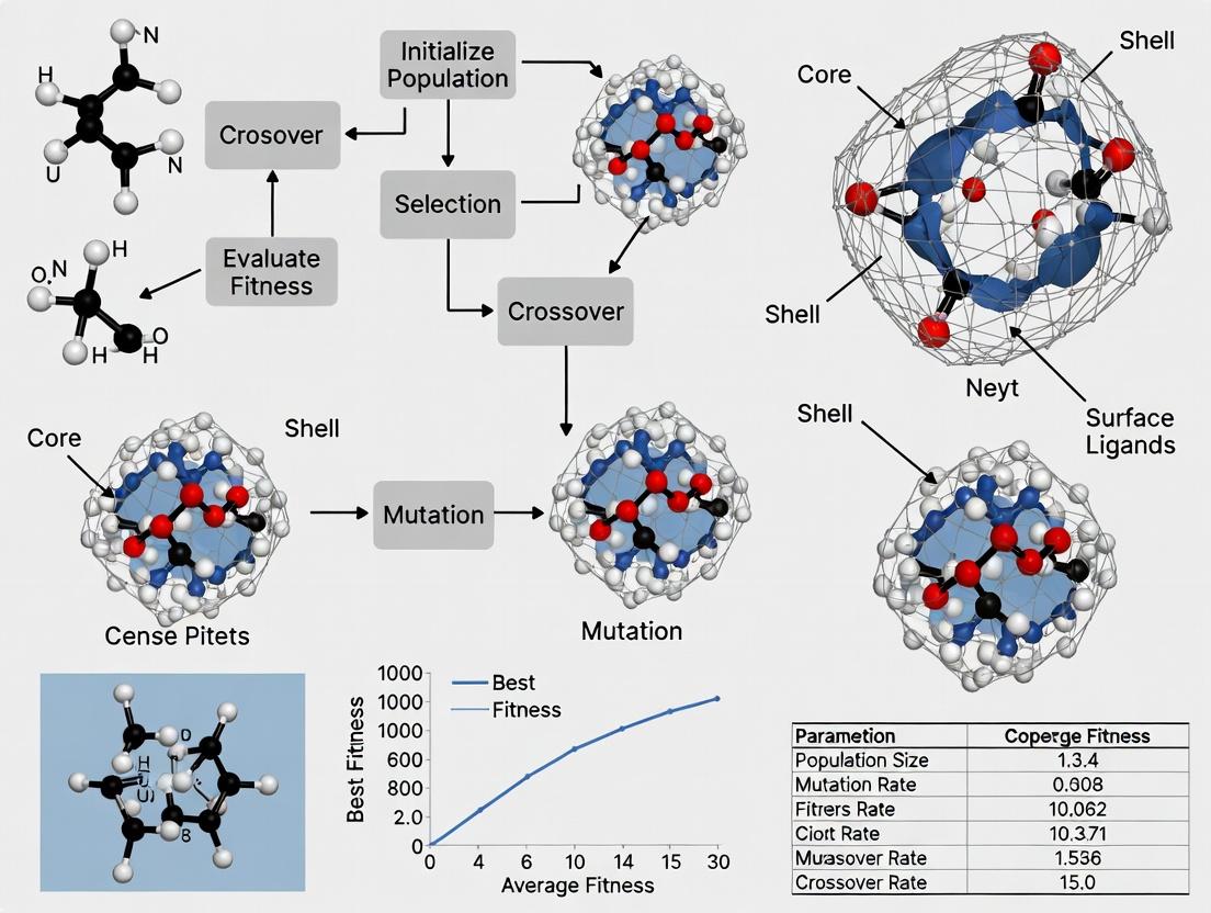
Visualization of Genetic Algorithm Workflow

Title: Genetic Algorithm Optimization Workflow for Nanoparticle Design

The Scientist's Toolkit: Key Research Reagent Solutions

Table 2: Essential Computational & Analytical Tools for GA-Driven Nanoparticle Research

Item / Solution	Function in GA Nanoparticle Optimization	Example/Note
Density Functional Theory (DFT) Software	Provides high-accuracy fitness evaluation via electronic structure calculations for stability, adsorption energies.	VASP, Quantum ESPRESSO, Gaussian. Critical for small clusters (<1000 atoms).
Molecular Dynamics (MD) Force Fields	Enables structural relaxation and dynamic property assessment of larger nanoparticles and ligand shells.	ReaxFF, CHARMM, GAFF. Used for pre-screening and validation.
Finite-Difference Time-Domain (FDTD) Solver	Computes optical properties (scattering, absorption) for plasmonic nanoparticle fitness evaluation.	Lumerical FDTD, MEEP. For noble metal and core-shell NPs.
High-Throughput Synthesis Robotics	Enables experimental validation and fitness measurement of GA-predicted optimal structures.	Liquid handling systems for automated colloidal synthesis.
Characterization Suite (In Silico & Experimental)	Validates predicted structures and measures fitness-relevant properties.	In Silico: VESTA (visualization). Experimental: TEM, XRD, DLS, UV-Vis spectroscopy.
GA/Evolutionary Algorithm Framework	Core platform for implementing selection, crossover, and mutation operators.	DEAP (Python), ParadisEO (C++), in-house MATLAB/Python code.
High-Performance Computing (HPC) Cluster	Executes parallel fitness evaluations (100s-1000s of simulations) required for GA population evolution.	Essential for practical runtime when using DFT/MD fitness functions.

Within the broader thesis on the Global optimization of nanoparticle structures with genetic algorithms, this document details the application notes and protocols for leveraging Genetic Algorithms (GAs) in nanostructure discovery. GAs are uniquely suited for navigating the complex, high-dimensional potential energy surfaces characteristic of nanomaterials, which are often riddled with discontinuities and multiple local minima (multi-modality). These landscapes challenge traditional gradient-based optimization methods, making population-based, evolutionary strategies a critical tool for identifying globally optimal or novel metastable nanostructures for applications in catalysis, drug delivery, and photonics.

Application Notes: Core Advantages & Quantitative Benchmarks

The following table summarizes key comparative studies highlighting the performance of GAs against other optimization methods in nanostructure discovery.

Table 1: Benchmark Performance of GAs on Nanostructure Optimization Problems

System/Objective (Reference)	Compared Methods	GA Performance Metric	Key Advantage Demonstrated
Au-Pt Core-Shell Nanoalloy Stability (DFT-based search, 2023)	Simulated Annealing (SA), Basin Hopping (BH)	Found 15% lower energy global min. vs. BH; 28% higher success rate over 50 runs vs. SA.	Superior global search in discontinuous compositional space.
Ligand Shell Optimization for Drug-Loaded Dendrimers (2024)	Random Search, Particle Swarm Optimization (PSO)	Achieved target binding affinity 2.3x faster (in generations) than PSO.	Efficient handling of discrete ligand type/position variables.
2D MoS2 Defect Engineering for Catalysis (2022)	Gradient Descent (GD), Monte Carlo (MC)	Identified 7 distinct low-energy defect configurations (multi-modal solutions) missed by GD.	Simultaneous mapping of multiple promising solution basins.
DNA Origami Folding Pathway (Coarse-grained MD, 2023)	Molecular Dynamics (MD) Quenching	Reduced required MD sampling steps by ~70% to find stable fold.	Effective steering of high-dimensional conformational searches.

Experimental Protocols

Protocol 3.1: GA-Driven Discovery of Bimetallic Nanoalloy Catalysts

Objective: To identify the globally minimum energy structure and composition of a 55-atom (PtxAu1-x)55 cluster for oxygen reduction reaction (ORR) activity. Materials: See Toolkit Section 4. Procedure:

• Encoding: Represent a candidate nanoparticle as a string of 55 integers. Each integer denotes an atom type (e.g., 0=Pt, 1=Au) and its relative 3D position is mapped via a fixed lattice (e.g., Mackay icosahedron).
• Initialization: Generate a random population of 100 candidates.
• Fitness Evaluation: Calculate the total energy using a pre-trained Machine Learning Force Field (MLFF) for rapid evaluation (~1-2 sec/structure). Fitness = -1 * (Total Energy).
• Selection: Perform tournament selection (size=3) to choose parents.
• Crossover: Apply a cut-and-splice operator: two parent clusters are cut at a random plane and recombined to produce two offspring, preserving total composition approximately.
• Mutation: Apply three mutation operators with defined probabilities:
  • Swap (P=0.7): Swap the positions of two randomly chosen atoms of different elements.
  • Strain (P=0.2): Randomly perturb the Cartesian coordinates of all atoms by a small Gaussian displacement (σ=0.1 Å).
  • Composition Change (P=0.1): Replace a random surface atom with the other element type.
• Replacement: Use an elitist strategy, replacing the worst 90% of the population with new offspring, retaining the top 10%.
• Termination: Run for 200 generations or until the best fitness remains unchanged for 20 generations.
• Validation: Re-evaluate the top 10 final structures using full DFT (e.g., VASP) to confirm stability and calculate ORR adsorption energies.

Protocol 3.2: Optimizing Lipid Nanoparticle (LNP) Formulations for mRNA Delivery

Objective: To optimize a multi-component LNP formulation (lipid ratios, polymer inclusion) for high mRNA encapsulation efficiency and cell-specific uptake. Encoding: A candidate is a vector of 5 continuous variables: molar ratios of ionizable lipid, phospholipid, cholesterol, PEG-lipid, and a targeting polymer weight percentage. Fitness Function: A weighted sum of in vitro outputs: Fitness = (0.4 * Encapsulation %) + (0.5 * Target Cell Uptake [flow cytometry MFI]) + (0.1 * (-1 * Cytotoxicity Score)). Procedure:

• Initial DoE: Use a space-filling design (e.g., Latin Hypercube) to generate the initial population of 50 formulations. Synthesize and characterize these LNPs.
• GA Loop: a. Evaluate fitness based on experimental data. b. Perform selection via rank-based roulette wheel. c. Apply blend crossover (BLX-α, α=0.5) for continuous variables. d. Apply Gaussian mutation (σ = 5% of variable range). e. Generate 20 new candidate formulations per generation.
• Parallel Experimentation: Synthesize and test the 20 new formulations in a single batch to maintain generational synchrony.
• Convergence: Run for 8-10 generations (~300 total experiments). The Pareto front of solutions balancing encapsulation and uptake is analyzed.

The Scientist's Toolkit

Table 2: Essential Research Reagent Solutions & Computational Tools

Item/Category	Function in GA-driven Nanostructure Discovery
MLFF Potentials (e.g., MACE, NequIP)	Provides near-DFT accuracy energy/force evaluations at ~10^5 speedup, enabling feasible fitness evaluation for thousands of candidates.
Atomic Simulation Environment (ASE)	Python framework for setting up, manipulating, running, and analyzing atomistic simulations; essential for integrating GA with DFT/MLFF calculators.
Deap or JGAP Libraries	Robust Python/Java frameworks for rapid implementation of custom GA operators, selection, and evolutionary loops.
High-Throughput Microfluidics Platform	For physical synthesis and screening of nanoparticle formulations (e.g., LNPs, quantum dots) defined by GA-generated parameter sets.
Cryo-EM/High-Res TEM Services	Critical validation step to resolve the atomic or morphological structure of top-predicted candidates from a GA search.

Visualization of Workflows

GA Optimization Loop for Nanostructures

GA vs GD on Rugged Landscape

Building Your Algorithm: A Step-by-Step Guide to GA-Driven Nanoparticle Optimization

Within the broader thesis on the global optimization of nanoparticle structures with genetic algorithms (GAs), the initial and most critical step is the development of a robust genotype representation. This encoding scheme must translate the complex, multi-parameter architecture of a nanoparticle—encompassing its physicochemical and biological properties—into a string of data (the genotype) that a GA can manipulate. An effective encoding balances expressiveness (ability to represent diverse, high-performing designs) with evolvability (allowing for meaningful crossover and mutation operations). This Application Note details current strategies and provides protocols for implementing nanoparticle genotype encoding for computational optimization.

Core Encoding Strategies

The choice of encoding scheme dictates the search space for the optimization algorithm. The table below summarizes the primary strategies, their applications, and key considerations.

Table 1: Nanoparticle Genotype Encoding Strategies

Encoding Type	Description	Best For	Advantages	Disadvantages	Key Parameters Encoded
Direct / Real-Valued	A vector of real numbers representing continuous design variables.	Lipid nanoparticles (LNPs), polymeric NPs with tunable continuous properties.	Intuitive, allows fine-grained optimization, efficient for continuous parameters.	May require boundary constraints; standard crossover/mutation may create invalid offspring.	Core diameter, polymer chain length, PEG density, lipid molar ratios, zeta potential target.
Binary	Design parameters converted to binary bit strings.	Discrete choices or coarsely discretized continuous variables.	Classic GA compatibility; simple crossover/mutation.	Limited precision for continuous variables; Hamming cliffs.	Material type selection, ligand presence/absence, surface coating type from a fixed list.
Integer / Categorical	Vector of integers representing selections from predefined lists or discrete counts.	Multi-layered or multi-component NPs with distinct material choices.	Natural for representing categorical choices and ordered layers.	Requires specialized genetic operators for categorical variables.	Layer sequence (e.g., core-shell), material ID per layer, number of targeting ligands.
Variable-Length / Tree-Based	Hierarchical or tree structure (e.g., LISP S-expressions).	Complex, modular architectures like dendrimers or branched structures.	Can represent hierarchical composition and topology; enables automated innovation of structure.	Complex implementation; requires robust operators to maintain tree validity.	Branching points, monomer types at nodes, polymer generation number, functional group placement.
Composite / Mixed	Hybrid of above types within a single genotype.	Most real-world nanoparticle designs (e.g., a targeted LNP).	Maximizes flexibility to represent heterogeneous parameter types.	Requires careful design of genetic operators for each segment.	[Real: core size] + [Integer: coating material] + [Binary: ligand flags] + [Real: ligand density].

Experimental Protocol: Designing a Composite Genotype for a Targeted Lipid Nanoparticle

This protocol outlines the steps to create a genotype for optimizing a siRNA-loaded, targeted LNP.

Protocol 3.1: Genotype Definition and Initialization

• Objective: To define a composite genotype representing a targeted LNP for a GA.
• Materials: Computational environment (Python with libraries like DEAP, NumPy), parameter definition file.
• Procedure:
  • Define Parameter Space: Specify all tunable variables with their types, ranges, or possible values.
    • Continuous (Real): Molar ratios of ionizable lipid (20-60%), helper lipid (20-50%), cholesterol (10-40%), PEG-lipid (0.5-5%). Total must equal 100%.
    • Continuous (Real): N/P ratio (2-10).
    • Categorical (Integer): Targeting ligand type (0: none, 1: folate, 2: RGD peptide, 3: aptamer).
    • Continuous (Real): Ligand density (0.1-5.0 mol% if ligand present).
  • Design Genotype Structure: Create a composite genotype as a list: [Lipid_Ratio_Vector, N_P_Ratio, Ligand_Type, Ligand_Density].
  • Implement a Custom Initialization Function:
    • For Lipid_Ratio_Vector, generate four random numbers, normalize to sum to 100%.
    • For N_P_Ratio, sample uniformly from [2, 10].
    • For Ligand_Type, assign 0 with 30% probability, else randomly choose 1, 2, or 3.
    • For Ligand_Density, if Ligand_Type > 0, sample from [0.1, 5.0]; else set to 0.

Protocol 3.2: Implementation of Custom Genetic Operators

• Objective: To ensure genetic operations produce valid, meaningful offspring genotypes.
• Procedure:
  • Crossover (Blend Crossover for Real, Uniform for Categorical):
    • For the Lipid_Ratio_Vector and N_P_Ratio, use simulated binary crossover (SBX) or blend crossover (BLX-α).
    • For Ligand_Type, use uniform crossover (randomly swap values between parents).
    • Apply a repair function post-crossover to re-normalize lipid ratios to 100%.
  • Mutation (Polynomial for Real, Random Reset for Categorical):
    • For real-valued genes, use polynomial mutation.
    • For Ligand_Type, with a small probability, randomly reset to a new valid value (including 0).
    • If Ligand_Type mutates to/from 0, adjust Ligand_Density accordingly (set to 0 or sample anew).
    • Re-normalize lipid ratios after mutation if they were altered.
  • Constraint Handling: Embed the normalization repair function within the operators to automatically satisfy the sum constraint.

Visualization: Encoding and Optimization Workflow

Diagram 1: Encoding's Role in GA-driven Nanoparticle Optimization

The Scientist's Toolkit: Research Reagent Solutions

Table 2: Essential Resources for Encoding and In Silico Optimization

Item / Solution	Function in Encoding & Optimization	Example / Note
Computational Framework (DEAP, JMetal)	Provides foundational tools for implementing GAs, including various selection, crossover, and mutation operators.	DEAP (Distributed Evolutionary Algorithms in Python) is highly flexible for custom genotype and operator design.
Chemical Database (PubChem, ZINC)	Sources for assigning categorical IDs to chemical components (e.g., lipid IDs, polymer SMILES strings) in the genotype.	PubChem CID can be an integer gene representing a specific lipid.
Property Predictor Library (RDKit, ChemAxon)	Used within the fitness function to predict physicochemical properties (LogP, molar refractivity) from a chemical structure ID in the genotype.	Enables preliminary fitness screening before experimental validation.
Constraint Handling Library (PyGMO, Custom)	Manages parameter constraints (e.g., sum of ratios = 100%) during genotype initialization and genetic operations.	Critical for maintaining valid, physically-realizable nanoparticle designs.
Data Serialization Format (JSON, XML)	Standardized format for saving, sharing, and reproducing the complete genotype definition and evolved populations.	Ensures reproducibility of the computational optimization experiment.

The encoding of nanoparticle architectures into a manipulatable genotype is the foundational step that bridges materials design and artificial evolution. A well-designed composite encoding scheme, coupled with tailored genetic operators, allows GAs to efficiently explore the vast, multi-dimensional design space of modern nanomedicines. The protocols and strategies outlined here provide a template for researchers to implement this critical first step within a global optimization pipeline, accelerating the discovery of next-generation nanoparticle therapeutics.

Within the global optimization of nanoparticle structures using genetic algorithms, the fitness function is the critical translator between computational simulation and biomedical efficacy. This protocol details the systematic construction of multi-objective fitness functions that quantitatively map in silico nanoparticle descriptors to quantifiable biological and therapeutic outcomes, enabling the algorithm to evolve designs toward clinically relevant goals.

The genetic algorithm's evolutionary drive is governed entirely by the fitness function. For nanoparticle optimization, this function must bridge multiple scales: from atomic-level molecular dynamics (MD) simulation outputs (e.g., binding energy, stability) to mesoscale pharmacokinetic (PK) properties (e.g., circulation time, biodistribution), and ultimately to macroscopic therapeutic outcomes (e.g., tumor regression, reduced toxicity). A poorly defined function yields optimized but therapeutically irrelevant structures.

Defining Biomedical Goal Metrics

Primary goals must be translated into quantifiable metrics suitable for computation.

Table 1: Core Biomedical Goals and Their Quantitative Proxies

Biomedical Goal	Quantitative Proxy Metric	Experimental Validation Method
Targeted Cellular Uptake	Specific binding free energy (ΔG, kcal/mol) to target vs. non-target receptors.	Surface Plasmon Resonance (SPR); Competitive cell binding assay.
Prolonged Circulation	Fraction of bound serum proteins (e.g., opsonins) from MD; Hydrodynamic diameter (nm).	Dynamic Light Scattering (DLS) in serum; PK studies in vivo.
Endosomal Escape	Pore formation energy in lipid bilayer; pKa of ionizable lipids.	Fluorescence co-localization assay (e.g., dye leakage); Hemolysis assay at pH 5.5.
Drug Release at Target	Trigger-responsive linker cleavage rate (ns^-1); Diffusion coefficient of payload.	Dialysis-based release kinetics under trigger (pH, enzyme, redox).
Minimized Toxicity	Interaction energy with critical off-target proteins (e.g., hERG); Complement activation score.	In vitro cytotoxicity (IC50); In vivo serum biomarker analysis (e.g., ALT, AST).

Constructing the Multi-Objective Fitness Function

A weighted sum approach is common, but requires careful normalization.

Fitness, F = Σ (wi * Ni(Si)) Where: wi = weight for objective i (Σwi = 1); Si = raw score from simulation/descriptor; Ni = normalization function mapping Si to a [0,1] scale.

Protocol 3.1: Defining Normalization Functions

• For "More is Better" goals (e.g., binding affinity):
  • N_i(S_i) = (S_i - S_min) / (S_max - S_min) if bounds are known.
  • Use a sigmoid function (1 / (1 + exp(-k*(S_i - S_thresh)))) if a threshold (S_thresh) exists, where k controls steepness.
• For "Less is Better" goals (e.g., toxicity score):
  • Invert the "More is Better" normalization: N_i(S_i) = 1 - [(S_i - S_min) / (S_max - S_min)].
• For "Target Range" goals (e.g., hydrodynamic diameter 50-150 nm):
  • Use a piecewise function that peaks at 1 within the ideal range and falls to 0 outside defined limits.

Protocol 3.2: Assigning Objective Weights via Analytic Hierarchy Process (AHP)

• Consult with biomedical collaborators to pairwise compare all objectives in Table 1.
• Use a standard 1-9 importance scale (1=equal importance, 9=extremely more important).
• Construct a reciprocal comparison matrix.
• Calculate the principal eigenvector of the matrix; this provides the weight vector w_i. This formalizes expert judgment into reproducible weights.

Experimental Validation Protocols for Fitness Components

Protocol 4.1: Validating Binding Affinity Predictions

• Objective: Correlate computed ΔG with experimental KD.
• Method (SPR):
  • Immobilize the target receptor on a CMS sensor chip via amine coupling.
  • Flow nanoparticle solutions at five concentrations (e.g., 0.5-50 nM) over the surface at 30 µL/min.
  • Record association (120 s) and dissociation (300 s) phases.
  • Fit sensorgrams to a 1:1 Langmuir binding model to obtain ka (association rate) and kd (dissociation rate). KD = kd/ka.
  • Perform linear regression between computed ΔG and -RT ln(KD).

Protocol 4.2: Validating Serum Stability & Opsonization

• Objective: Correlate MD-derived protein corona profiles with experimental size increase.
• Method (DLS in Serum):
  • Incubate nanoparticle formulation (1 mg/mL) in 90% FBS at 37°C.
  • At time points (0, 1, 4, 24 h), dilute sample 1:50 in PBS.
  • Measure hydrodynamic diameter (Z-avg) and PDI via DLS (3 measurements of 15 runs each at 25°C).
  • The slope of diameter increase over the first 4 hours serves as the experimental stability score.

Table 2: Research Reagent Solutions Toolkit

Reagent / Material	Function in Validation	Key Considerations
CMS Sensor Chip (e.g., Cytiva)	SPR substrate for immobilizing biomolecular targets.	Ensures consistent, low-nonspecific binding surface for kinetics.
Human Serum Albumin (HSA)	Major serum protein for corona and stability studies.	Use fatty-acid-free for consistent initial binding conditions.
FRET-based Lipid Nanoparticles	Contain donor/acceptor dyes to monitor integrity and fusion.	Enables real-time, quantitative tracking of payload release.
hERG-Expressing Cell Line (e.g., HEK293)	In vitro model for assessing cardiac toxicity potential.	Critical for evaluating off-target interactions predicted by MD.
pH-Sensitive Dye (e.g., LysoTracker)	Fluorescent marker for tracking endosomal localization/escape.	Validates predictions of endosomal escape efficiency.

Integration Workflow Diagram

Fitness Function Workflow in GA Optimization

Case Example: Optimizing an siRNA-LNP for Liver Delivery

Goals: 1) Maximize hepatocyte uptake (via ApoE-mediated targeting), 2) Maximize endosomal escape, 3) Minimize spleen sequestration.

Constructed Fitness Function: F = 0.5 * N_binding(ΔG_ApoE) + 0.3 * N_escape(Pore_Energy) + 0.2 * (1 - N_spleen(Spleen_Accumulation_Score))

Validation Results:

• Generation 1 (Random): Average F = 0.42. In vivo: 5% liver siRNA dose, high spleen.
• Generation 15 (Optimized): Average F = 0.86. In vivo: 55% liver siRNA dose, 3-fold lower spleen.

The fitness function is the embodiment of the research hypothesis within the optimization loop. Its careful construction, grounded in validated quantitative proxies for biomedical goals, is the single most important step in ensuring that a globally optimized nanoparticle structure is not just computationally elegant, but therapeutically potent.

This protocol details the configuration of evolutionary operators for the global optimization of metallic and bimetallic nanoparticle structures using genetic algorithms (GAs). Within the broader thesis on "Global optimization of nanoparticle structures with genetic algorithms research," this step is critical for navigating the complex, high-dimensional search space of atomic coordinates, composition, and morphology to identify nanoparticles with target properties such as catalytic activity or plasmonic response.

Core Evolutionary Operators: Configuration & Rationale

Evolutionary operators drive the exploration and exploitation of the structural search space. Their parameters must be tuned for the specific domain of nanoparticle optimization.

Table 1: Configured Evolutionary Operators and Parameters

Operator Category	Specific Operator	Typical Parameter Range	Rationale for Nanoparticle Search
Selection	Tournament Selection	Tournament Size: 3-5	Maintains selection pressure while preserving diversity. Favors fitter structures for reproduction.
Selection	Fitness Proportionate (Roulette Wheel)	–	Rarely used due to premature convergence in complex search spaces.
Crossover	Cut-and-Splice (for NPs)	Probability: 0.6-0.8	Swaps clusters of atoms between two parent structures. Crucial for exploring hybrid morphologies.
Crossover	Homologous Crossover	Probability: 0.7-0.9	Aligns parent structures by symmetry or center of mass before exchanging atoms. Better for local refinement.
Mutation	Atom Displacement	Probability: 0.1-0.3; Max Displacement: 0.5-1.5 Å	Introduces local relaxations and defects, preventing stagnation in local minima.
Mutation	Composition Swap (for bimetallics)	Probability: 0.05-0.15	Randomly swaps atom identities (e.g., Pt and Au) to optimize alloy distribution.
Mutation	Rotation/Translation	Probability: 0.05-0.1	Rotates or translates sub-clusters within the nanoparticle.
Fitness Evaluation	DFT (High Accuracy)	–	Used for final candidate validation. Computationally expensive.
Fitness Evaluation	Machine Learning Potentials/Surrogates	–	Used during GA evolution for rapid screening of thousands of structures.

Detailed Experimental Protocol: A Single GA Cycle for Nanoparticle Optimization

Protocol: One Iteration (Generation) of the Genetic Algorithm Objective: To evolve a population of nanoparticle structures toward lower adsorption energies for a target molecule (e.g., O₂, CO) or higher stability.

Materials & Reagents:

• Initial Population: A set of 30-50 nanoparticle structures (typically 50-200 atoms each) generated via random seeding, known motifs (icosahedron, decahedron, FCC), or previous simulations.
• Computational Software: GA framework (e.g., ASE, GASP, custom Python), energy calculator (DFT code like VASP or Quantum ESPRESSO, or a pre-trained ML potential).
• Fitness Metric Script: Code to compute the property of interest (e.g., adsorption energy, cohesive energy, HOMO-LUMO gap) from the calculator output.

Procedure:

• Fitness Evaluation: a. For each structure in the current population, perform a local geometry relaxation using the chosen energy calculator (ML potential recommended for speed). b. Compute the target fitness property (e.g., Eads = E(NP+adsorbate) - ENP - Eadsorbate). c. Rank the entire population from best (e.g., most negative E_ads) to worst.

• Selection: a. Employ tournament selection (size=4). b. Randomly pick 4 structures from the population. Select the one with the best fitness as Parent A. c. Repeat the process to select Parent B.

• Crossover (Cut-and-Splice): a. Generate a random number r between 0 and 1. If r < Crossover Probability (e.g., 0.7), proceed. b. For Parent A and B, randomly select a cutting plane in 3D space. c. Create Child by taking atoms from one side of the plane from Parent A and atoms from the other side from Parent B. d. Resolve any severe atomic clashes with a quick partial relaxation.

• Mutation (Probabilistic Application): a. For the new Child structure, generate a new random number s for each mutation operator. b. If s < Displacement Mutation Probability (0.2): Randomly displace ~10% of its atoms by a random vector (max length 1.0 Å). c. If s < Swap Mutation Probability (0.1) and NP is bimetallic: Randomly select 2-5 pairs of unlike atoms and swap their identities. d. Relax the mutated child structure briefly.

• Replacement (Elitist Strategy): a. Insert the new Child into a "next generation" pool. b. Repeat Steps 2-4 until the next generation pool is full. c. Copy the top 2-3 structures (elites) from the current generation directly into the next generation, replacing the worst offspring.

• Iteration: Designate the new pool as the current population. Return to Step 1. Continue for 50-200 generations or until convergence (no improvement in best fitness for 20 generations).

The Scientist's Toolkit: Key Research Reagent Solutions

Table 2: Essential Computational Tools for GA-Driven Nanoparticle Search

Item/Software	Function & Rationale
Atomic Simulation Environment (ASE)	Python library for setting up, manipulating, running, visualizing, and analyzing atomistic simulations. Essential for building the GA workflow.
VASP/Quantum ESPRESSO	High-accuracy DFT calculators. Used for final validation and for generating training data for ML potentials.
Machine Learning Potentials (e.g., M3GNet, NequIP)	Surrogate models trained on DFT data. Enable rapid energy/force calculations, making evolution of large populations feasible.
OVITO	Visualization and analysis software for atomistic data. Critical for inspecting evolved nanoparticle morphologies.
PyMatgen	Python materials analysis library. Useful for analyzing structural features, symmetry, and composition of generated NPs.
Custom Python GA Script	Orchestrates selection, crossover, mutation, and fitness evaluation by integrating the above tools.

Workflow & Pathway Visualizations

Operator Decision Logic for Nanoparticle Mutation

This case study is positioned within a doctoral thesis focused on the global optimization of nanoparticle structures with genetic algorithms (GAs). LNPs represent a complex, high-dimensional formulation space where four primary lipid components interact non-linearly to determine efficacy and safety. Traditional one-variable-at-a-time experimentation is inefficient for navigating this space. This protocol details an integrated approach where a GA is employed to efficiently search and identify optimal LNP compositions for mRNA delivery, iteratively guided by high-throughput in vitro screening data.

Core Protocol: GA-Driven LNP Formulation Screening

Objective

To identify an LNP formulation that maximizes mRNA translation efficiency (luciferase expression) in HepG2 cells while minimizing cytotoxicity, using a GA to optimize the molar ratios of four lipid components.

Detailed Experimental Methodology

Step 1: Define the Genetic Algorithm Parameters

• Gene Representation: Each LNP formulation ("individual") is represented as a set of four continuous genes corresponding to molar percentages:
  • Gene 1: Ionizable Cationic Lipid (ICL)
  • Gene 2: Phospholipid (DSPC)
  • Gene 3: Cholesterol (Chol)
  • Gene 4: PEGylated Lipid (PEG-lipid)
  • Constraint: ICL + DSPC + Chol + PEG-lipid = 100 mol%
• Initial Population (Generation 0): N=50 random formulations satisfying the molar sum constraint.
• Fitness Function: F = log10(Total Luciferase Expression in RLU) - 5*(Cell Viability Fraction - 0.9)^2. This prioritizes high expression but penalizes viability below 90%.
• Selection: Tournament selection (size=3).
• Crossover: Blend crossover (BLX-α, α=0.5) applied to parent pairs.
• Mutation: Gaussian noise (σ = 2 mol%) applied to a random gene in 20% of offspring, followed by re-normalization to 100 mol%.
• Elitism: Top 2 formulations carried over to next generation.
• Termination: After 15 generations or upon fitness plateau.

Step 2: High-Throughput LNP Formulation (Microfluidics)

• Lipid Stock Solution: Prepare each lipid in ethanol at a combined concentration of 12.5 mM total lipid.
• Aqueous Phase: Dilute mRNA (e.g., firefly luciferase) in 50 mM citrate buffer (pH 4.0) to 0.1 mg/mL.
• Mixing: Use a staggered herringbone micromixer chip or commercial equivalent (e.g., NanoAssemblr).
  • Set Total Flow Rate (TFR) to 12 mL/min.
  • Set Aqueous-to-Organic Flow Rate Ratio (FRR) to 3:1.
  • Collect LNPs in a vessel containing 4x volume of 1x PBS (pH 7.4) for buffer exchange.
• Characterization: For each formulation in a generation, measure particle size (Z-average, PDI) and zeta potential via dynamic light scattering (DLS).

Step 3: In Vitro Screening for Fitness Evaluation

• Cell Seeding: Seed HepG2 cells in 96-well plates at 10,000 cells/well in complete media. Incubate for 24 h.
• Dosing: Apply LNPs containing 50 ng mRNA per well. Include controls (untreated cells, naked mRNA). Incubate for 24 h.
• Viability Assay (MTS): Aspirate media, add fresh media with MTS reagent (20% v/v). Incubate 1-2 h, measure absorbance at 490 nm. Calculate viability relative to untreated cells.
• Luciferase Expression Assay: Lyse cells with 1x Passive Lysis Buffer for 15 min. Mix luciferase assay reagent with lysate, measure luminescence (RLU) on a plate reader.
• Fitness Score Calculation: Compute fitness F for each LNP formulation using the function above. This data feeds back into the GA to create the next generation.

Table 1: Key Physical Characteristics of Top-Performing LNP Formulations Identified by GA

Generation	Formulation ID (ICL:DSPC:Chol:PEG)	Size (nm)	PDI	Zeta Potential (mV)	Luciferase RLU (x10^9)	Cell Viability (%)	Fitness Score (F)
0 (Random)	F0-12 (50:10:38.5:1.5)	145	0.12	-2.1	1.2	85	8.70
5	F5-03 (45:12:41.5:1.5)	112	0.08	-1.8	5.8	92	9.74
10	F10-01 (40:15:43:2)	95	0.06	-3.5	9.5	96	9.96
15 (Final)	F15-07 (38:16:44:2)	88	0.05	-4.2	12.4	98	10.09

Table 2: Genetic Algorithm Optimization Parameters and Outcomes

Parameter	Value Set	Outcome Metric	Final Value
Population Size	50	Generations to Convergence	14
Crossover Rate	80%	Best Fitness (Generation 0)	8.70
Mutation Rate	20%	Best Fitness (Final)	10.09
Elite Count	2	Avg. Fitness Improvement	+16%

The Scientist's Toolkit: Key Research Reagent Solutions

Item	Function in LNP Optimization	Example/Note
Ionizable Cationic Lipid (ICL)	Encapsulates mRNA via electrostatic interaction; fuses with endosomal membrane for release.	SM-102, ALC-0315. Critical for endosomal escape.
Phospholipid (Helper Lipid)	Provides structural integrity to the LNP bilayer; influences fusogenicity.	DSPC, DOPE. DSPC enhances stability.
Cholesterol	Stabilizes LNP structure and enhances membrane fusion.	Often used at ~40 mol%. Essential for in vivo efficacy.
PEGylated Lipid	Shields LNP surface, reduces aggregation, modulates pharmacokinetics.	DMG-PEG2000, ALC-0159. Impacts cellular uptake.
Microfluidic Mixer	Enables reproducible, rapid mixing for precise LNP self-assembly.	NanoAssemblr, PDMS-based staggered herringbone chip.
Luciferase Reporter mRNA	Quantifiable payload to measure delivery and functional protein expression.	CleanCap modified mRNA with pseudouridine.
Cell Viability Assay Kit	High-throughput metabolic assay to quantify formulation cytotoxicity.	MTS or CellTiter-Glo assays.
Dynamic Light Scattering (DLS) Instrument	Measures LNP hydrodynamic diameter, polydispersity (PDI), and zeta potential.	Malvern Zetasizer Nano ZS.

Visualization of Workflows and Pathways

GA-LNP Optimization Workflow

LNP-mRNA Endosomal Escape Pathway

This case study demonstrates the practical application of global optimization frameworks, central to the thesis on Global optimization of nanoparticle structures with genetic algorithms research. Photothermal therapy (PTT) requires nanoparticles (NPs) with maximized photothermal conversion efficiency (PCE), a complex function of geometry, composition, size, and surface chemistry. Empirical design is inefficient. Here, genetic algorithms (GAs) are employed to navigate this high-dimensional parameter space, evolving nanoparticle populations toward optimal PTT performance as defined by a multi-objective fitness function.

Core Optimization Parameters & Quantitative Data

The genetic algorithm operates on a genome encoding key nanoparticle attributes. The fitness function evaluates candidates based on the following simulated or experimentally measured parameters.

Table 1: Genetic Algorithm Genome Encoding for PTT Nanoparticle Design

Gene Parameter	Encoding Range	Description
Core Material	{Au, Ag, Pd, Pt, Au-Ag Alloy}	Plasmonic metal determining initial LSPR peak.
Core Geometry	{Sphere, Rod, Shell, Cube, Star}	Shape drastically influences scattering/absorption ratio and field enhancement.
Characteristic Size (nm)	10 - 150 nm	Governs LSPR wavelength and biodistribution.
Aspect Ratio (for rods)	1.0 - 5.0	Fine-tunes longitudinal LSPR into NIR-I/II windows.
Shell Material/Thickness	{SiO₂: 5-30nm, PEG: 2-10nm}	Impacts biocompatibility, stability, and functionalization.
Surface Ligand Density	0.1 - 5.0 molecules/nm²	Affects cellular uptake and colloidal stability.

Table 2: Target Fitness Function Objectives & Weights

Objective	Metric	Target	Weight in GA
Optical Performance	Photothermal Conversion Efficiency (PCE, η)	Maximize (>70%)	0.35
Biological Window	LSPR Peak Wavelength (λ_max)	750 - 1100 nm	0.25
Photostability	PCE Degradation after 10 laser cycles	Minimize (<5%)	0.20
Cytotoxicity (baseline)	Cell Viability without laser (24h)	>90%	0.15
Scalability Index	Synthetic Yield & Reproducibility Score	Maximize	0.05

Experimental Protocol: Synthesis & Characterization of GA-Optimized Nanoparticles

Protocol 1: Seed-Mediated Growth for Optimized Gold Nanorods (GNRs) This protocol is derived from the GA output suggesting high-aspect-ratio GNRs with a thin PEG shell for target λ_max ~850 nm.

Materials:

• HAuCl₄·3H₂O, Hexadecyltrimethylammonium bromide (CTAB), Sodium borohydride (NaBH₄), Silver nitrate (AgNO₃), Ascorbic acid, mPEG-Thiol (5 kDa).
• NIR Laser (808 nm, 2 W/cm² adjustable), UV-Vis-NIR Spectrophotometer, TEM, Thermocouple.

Procedure:

• Seed Solution: Mix CTAB (5 mL, 0.20 M) with HAuCl₄ (5 mL, 0.50 mM). Add ice-cold NaBH₄ (0.60 mL, 0.010 M) under vigorous stirring for 2 min. Age at 28°C for 30 min.
• Growth Solution: Combine CTAB (40 mL, 0.10 M), HAuCl₄ (2.0 mL, 10 mM), AgNO₃ (0.8 mL, 10 mM), and Ascorbic acid (0.32 mL, 0.10 M). The GA-prescribed Ag⁺ volume determines aspect ratio.
• Initiate Growth: Add Seed Solution (96 μL) to the Growth Solution. Invert gently for 10 sec, then let rest undisturbed at 30°C for 12 h.
• PEGylation: Centrifuge GNRs at 12,000 rpm for 15 min. Resuspend pellet in 1 mL DI water. Add mPEG-Thiol at GA-optimized molar excess (e.g., 5000:1 PEG:Au). Stir gently for 24 h at RT.
• Purification: Centrifuge and resuspend in PBS (pH 7.4). Filter through a 0.45 μm membrane.

Protocol 2: In Vitro Photothermal Efficacy & Cytotoxicity Assay

Procedure:

• Cell Seeding: Plate 4T1 (murine breast cancer) cells in 96-well plates at 10⁴ cells/well. Incubate for 24 h.
• NP Incubation: Add GA-optimized NPs at a concentration gradient (0, 10, 25, 50 pM) to culture media. Incubate for 6 h.
• Photothermal Treatment: Replace media with fresh PBS. Irwellate cells with an 808 nm laser at 2 W/cm² for 5 min. Control wells are shielded. Monitor temperature with a calibrated IR camera.
• Viability Assessment: Post-irradiation, replace PBS with media containing MTT reagent (0.5 mg/mL). Incubate for 4 h. Solubilize formazan crystals with DMSO. Measure absorbance at 570 nm.
• Data Analysis: Calculate PCE (η) using the established energy balance model: η = (hSΔTmax - Qdis) / I(1 - 10^-Aλ), where h is heat transfer coefficient, S is surface area of the cell, ΔTmax is max temp change, Qdis is heat from solvent, I is laser power, Aλ is absorbance at 808 nm.

The Scientist's Toolkit: Key Research Reagent Solutions

Table 3: Essential Reagents for Metallic PTT Nanoparticle Research

Reagent/Material	Function	Key Consideration
Chloroauric Acid (HAuCl₄)	Gold precursor for synthesis of Au NPs.	High purity (>99.9%) ensures reproducible morphology.
Cetyltrimethylammonium Bromide (CTAB)	Shape-directing surfactant for anisotropic growth (e.g., rods).	Cytotoxic; must be thoroughly replaced post-synthesis.
mPEG-Thiol (various MW)	Provides "stealth" properties, reduces opsonization, enhances circulation time.	Thiol group binds Au; PEG chain length affects pharmacokinetics.
MTT Cell Viability Assay Kit	Standard colorimetric test for metabolic activity post-PTT treatment.	Formazan solubility is critical for accurate OD measurement.
NIR Laser (808 nm)	Light source for exciting nanoparticle LSPR in the biological window.	Precise power calibration and uniform beam profile are mandatory.
Indocyanine Green (ICG)	Reference molecule for comparative PCE studies.	Unstable in aqueous solution; use as a fresh control.

Visualizations

Title: Genetic Algorithm Workflow for PTT Nanoparticle Design

Title: Photothermal Cell Ablation Mechanism

Overcoming Computational Hurdles: Practical Tips for Efficient and Effective GA Runs

Within the broader research on Global optimization of nanoparticle structures with genetic algorithms, premature convergence and loss of genetic diversity are critical failures. These phenomena cause the algorithm to settle on suboptimal nanoparticle configurations (e.g., ligand shell arrangements, core geometries) that may have favorable local energy but miss the globally optimal structure with superior drug-loading capacity, targeting efficiency, or stability. This document provides application notes and protocols for detecting and mitigating these issues.

Detection Methods: Protocols and Data

Protocol 1.1: Monitoring Population Diversity Metrics

Objective: Quantitatively track the loss of diversity in the genetic algorithm (GA) population over generations. Materials: GA population data (genotypes/fitness values), computational analysis script. Procedure:

• Genotypic Diversity: Calculate the average Hamming distance between all pairs of individuals in the population for each generation. For real-valued encodings (e.g., nanoparticle atom coordinates), use the average Euclidean distance in parameter space.
• Phenotypic Diversity: Track the standard deviation of fitness values within the population for each generation.
• Gene Frequency: Monitor the allele (parameter value) distribution for key decision variables across the population.
• Best/Worst/Average Fitness: Record the trajectory of these three metrics.

Expected Output: Tables and plots showing the decline of diversity metrics alongside the convergence of fitness values.

Table 1.1: Key Metrics for Detecting Premature Convergence

Metric	Formula/Description	Threshold Indicator of Premature Convergence
Avg. Hamming Distance	(ΣᵢΣⱼ HammingDist(Indᵢ, Indⱼ)) / Nᵢⱼ	Rapid drop to near-zero values in early generations (<20% of total).
Fitness Std. Dev.	σ(Fitness₁, Fitness₂, ... Fitnessₙ)	σ approaches zero while best fitness is still far from theoretical or estimated optimum.
Best/Avg. Fitness Ratio	Fitnessbeₛₜ / Fitnessavg	Ratio approaches 1.0 (population homogenizes) prematurely.
Allele Fixation Rate	% of loci where >95% of population shares the same allele.	Fixation occurs in >70% of loci before generation G/2 (where G is max generations).

Protocol 1.2: Fitness Landscape Ruggedness Analysis

Objective: Estimate the difficulty of the optimization problem to anticipate convergence behavior. Materials: Selected nanoparticle candidate structures, local search algorithm (e.g., steepest descent). Procedure:

• From the final GA population, select the top 10 individuals and 10 random individuals.
• For each selected individual, perform a short, intense local search (e.g., 100 steps of conjugate gradient minimization on the energy landscape).
• Record the fitness improvement and the distance in parameter space the individual moved.
• If local searches from diverse starting points all converge to the same or very similar fitness basins, the landscape may be deceptive, encouraging premature convergence.

Table 1.2: Ruggedness Analysis Results Interpretation

Observation	Implication for GA
High improvement from diverse starts, converging to different optima.	Rugged landscape; diversity maintenance is crucial.
Low improvement from diverse starts, all converging to near-identical point.	Smooth, funnel-like landscape; premature convergence risk is high if selection pressure is strong.
High improvement only from top individuals, random ones show no progress.	Landscape has flat regions; diversity helps escape plateaus.

Mitigation Strategies: Protocols

Protocol 2.1: Adaptive Niching with Fitness Sharing

Objective: Maintain subpopulations in different peaks of the fitness landscape. Methodology:

• Calculate Niche Count: For each individual i, calculate its niche count m_i = Σⱼ sh(dᵢⱼ), where sh(d) is a sharing function (typically 1 if d < σ_share, else 0). dᵢⱼ is the genotypic distance.
• Adjust Fitness: Compute the shared fitness: F_shared(i) = F_raw(i) / m_i.
• Selection: Perform selection based on F_shared. This reduces the reproductive advantage of individuals in crowded niches.
• Parameters: σ_share (niche radius) must be tuned based on the expected number of optima in the nanoparticle design space.

Title: Adaptive Niching with Fitness Sharing Workflow

Protocol 2.2: Adaptive Operator and Parameter Control

Objective: Dynamically adjust mutation rates and operator probabilities based on population diversity. Methodology:

• Monitor Diversity: Use metrics from Protocol 1.1 (e.g., Fitness Std. Dev.) as feedback.
• Adjust Mutation Rate (p_m): Implement a rule: if diversity < threshold θ, then p_m = p_m * (1 + α), capped at a maximum (e.g., 0.3). If diversity is high, p_m can decay to a base minimum (e.g., 0.01).
• Adjust Crossover/Selection Pressure: Similarly, increase the probability of diversity-introducing operators (e.g., uniform crossover) when diversity is low. Reduce elitism percentage temporarily.

Title: Adaptive Parameter Control Feedback Loop

The Scientist's Toolkit: Research Reagent Solutions

Table 2: Essential Computational Tools for Nanoparticle GA Research

Item / Solution	Function in Experiment	Example / Note
Molecular Dynamics (MD) Engine	Provides the fitness function (energy evaluation) for candidate nanoparticle structures.	GROMACS, LAMMPS, AMBER. Critical for accurate scoring.
Genetic Algorithm Library	Core framework for population management, selection, crossover, and mutation operators.	DEAP (Python), GALib (C++). Customizable for nanoparticle encoding.
Structure Visualization Software	Visual inspection of converged structures and diversity of shapes/arrangements.	VMD, PyMol, ChimeraX. Essential for phenotypic analysis.
High-Performance Computing (HPC) Cluster	Enables parallel fitness evaluation of hundreds of nanoparticle candidates per generation.	SLURM-managed cluster with GPU nodes. Required for practical runtime.
Diversity Analysis Scripts	Custom scripts to calculate Hamming distance, allele frequency, and other metrics from Protocol 1.1.	Python (NumPy, Pandas). Must be tailored to the specific genome encoding.
Local Search Optimizer	Used for fitness landscape analysis (Protocol 1.2) and hybrid GA-local search strategies.	SciPy optimizers, custom gradient descent for force fields.

Within the thesis context of global optimization of nanoparticle structures with genetic algorithms (GAs), the strategic management of exploration and exploitation is paramount. This document outlines Application Notes and Protocols for implementing adaptive operator rate control, a method to dynamically balance the application of genetic operators (e.g., crossover, mutation) based on their recent performance, thereby enhancing the search for optimal nanoparticle configurations in drug delivery and therapeutic applications.

Table 1: Common Genetic Operators for Nanoparticle Optimization

Operator Type	Typical Rate Range (Static)	Primary Function	Role in Exploration/Exploitation
Crossover	60% - 80%	Combines genetic material from two parent structures.	High exploitation of existing good building blocks.
Mutation	1% - 20%	Introduces random changes to a single structure.	High exploration of new regions of the search space.
Local Search	5% - 30%	Refines a structure towards a local optimum.	Pure exploitation.
Duplication	0% - 10%	Copies high-fitness structures unchanged.	Maintains exploitation.

Table 2: Performance Metrics for Operator Adaptation

Metric	Formula/Description	Adaptation Rule Trigger
Operator Productivity	(Fitness Improvement attributed to operator) / (Times operator applied)	Increase rate if productivity is high relative to others.
Diversity Contribution	1 - (Avg. similarity of offspring to population)	Increase rate if contribution is high and population diversity is low.
Success Rate	(# Improved offspring) / (# Total offspring generated)	Modulate rate proportionally to success rate.

Experimental Protocols

Protocol 3.1: Implementing an Adaptive Rate GA for Lipid Nanoparticle (LNP) Formulation

Objective: To dynamically optimize LNP parameters (lipid ratios, PEGylation degree, cholesterol content) for maximal membrane fusion efficiency and payload capacity.

Materials:

• Initial Population: 200 LNP formulations defined by a real-valued genome [A, B, C, D] representing molar ratios.
• Fitness Function: Calculated in silico via coarse-grained molecular dynamics (CG-MD) score predicting fusion efficiency and stability.
• Genetic Operators: Simulated Binary Crossover (SBX), Polynomial Mutation, a local gradient-ascent search.
• Software: Custom Python GA framework (e.g., DEAP) integrated with MD simulation software (e.g., GROMACS).

Procedure:

• Initialization: Set initial operator rates: Crossover (Pc=0.7), Mutation (Pm=0.1), Local Search (Pl=0.05). Define a sliding window of 50 generations for performance tracking.
• Evaluation: For each generation, evaluate fitness of all new LNP structures using the CG-MD scoring function.
• Operator Tagging: Tag each new offspring with the identifier of the primary operator that created it.
• Performance Calculation (Every N generations): a. For each operator i, calculate its Success Rate (SR_i) over the last window. b. Compute the relative performance: RP_i = SR_i / (Σ SR_all_operators).
• Rate Adaptation (Every N generations): a. Update each rate: Rate_i(new) = Rate_i(old) * (1 - α) + (RP_i * α), where α (e.g., 0.2) is the adaptation strength. b. Normalize rates to sum to a constant (e.g., 0.85), reserving 15% for elite preservation.
• Selection & Iteration: Select the next generation using tournament selection. Return to Step 2 for 500 generations or until convergence.
• Validation: Synthesize top 5 in silico predicted LNPs and validate fusion efficiency in vitro.

Protocol 3.2: Benchmarking Adaptive vs. Static Rates

Objective: To quantitatively compare the performance of adaptive operator strategies against static baselines.

Procedure:

• Define Benchmark: Use a known nanoparticle optimization problem (e.g., gold nanocluster stability) with a computationally cheap surrogate fitness model.
• Experimental Arms:
  • Arm A: Static high-exploitation (Pc=0.8, Pm=0.05).
  • Arm B: Static high-exploration (Pc=0.5, Pm=0.3).
  • Arm C: Adaptive rates using the method in Protocol 3.1.
• Execution: Run 30 independent trials of each arm for 1000 generations.
• Data Collection: Record for each trial: Best Fitness per generation, Population Diversity Index, and time to reach 90% of global optimum.
• Analysis: Perform statistical comparison (e.g., Mann-Whitney U test) on final fitness values and convergence speed across arms.

Visualization: Workflows & Logic

Title: Adaptive Operator Rate GA Workflow

Title: Adaptive Rate Decision Logic

The Scientist's Toolkit

Table 3: Key Research Reagent Solutions for Nanoparticle GA Optimization

Item / Solution	Function in Research	Example / Specification
High-Throughput In Silico Library	Provides initial candidate structures and defines the genomic representation.	Lipid Database (LIPID MAPS), Cambridge Structural Database (CSD) for core templates.
Surrogate Fitness Model	Rapidly approximates nanoparticle performance to make GA evolution feasible.	Machine Learning model (e.g., Random Forest) trained on molecular descriptors and in vitro data.
Coarse-Grained Molecular Dynamics (CG-MD) Software	Provides high-fidelity fitness evaluation for key candidates.	Software: GROMACS, LAMMPS with MARTINI force field.
Genetic Algorithm Framework	Core engine for implementing selection, operators, and adaptation logic.	Python: DEAP, PyGAD, or custom NumPy-based framework.
High-Performance Computing (HPC) Cluster	Enables parallel fitness evaluation of population individuals.	Essential for integrating with CG-MD simulations.
In Vitro Validation Assay Kit	Ground-truth validation of top in silico optimized nanoparticle designs.	e.g., Membrane Fusion Assay Kit (fluorometric), DLS for size/PDI, HPLC for encapsulation efficiency.

This document serves as an application note and protocol for managing the high computational costs associated with the global optimization of nanoparticle (NP) structures using Genetic Algorithms (GAs). Within the broader thesis on "Global optimization of nanoparticle structures with genetic algorithms," a primary challenge is the prohibitive expense of repeatedly evaluating candidate NP structures via high-fidelity, quantum-mechanical simulations (e.g., Density Functional Theory). This note details the implementation of hybrid models and surrogate-assisted evolutionary strategies to dramatically accelerate the search for optimal NP geometries, compositions, and surface functionalizations relevant to drug delivery and catalytic applications.

Core Methodologies: Protocols and Application Notes

Protocol: Implementation of a Surrogate-Assisted Genetic Algorithm (SAGA)

Objective: To reduce the number of costly DFT evaluations by iteratively training a surrogate model on a subset of evaluated candidates.

Materials & Computational Environment:

• High-Performance Computing (HPC) cluster.
• DFT software (e.g., VASP, Quantum ESPRESSO).
• Machine Learning library (e.g., Scikit-learn, TensorFlow).
• Custom Python scripting for GA and surrogate integration.

Procedure:

• Initial Sampling: Generate an initial population of N=100 candidate NP structures using a space-filling design (e.g., Latin Hypercube Sampling) across the defined search space (e.g., size, shape, dopant positions).
• High-Fidelity Evaluation: Perform full DFT relaxation and property calculation (e.g., adsorption energy, HOMO-LUMO gap) on the initial population. Store results in database DB1.
• Surrogate Model Training: Train a Gaussian Process Regressor (GPR) or a Neural Network on DB1. The model inputs are structural descriptors; the output is the target property.
• Evolutionary Cycle: a. Run a standard GA (selection, crossover, mutation) for G=50 generations. Evaluate the fitness of all offspring using the surrogate model. b. From the final surrogate-evaluated generation, select the top M=10 most promising and diverse candidates (using a diversity measure like crowding distance). c. Perform high-fidelity DFT evaluation on these M candidates. d. Add the new (structure, property) pairs to DB1 and retrain the surrogate model.
• Convergence Check: Repeat Step 4 until the improvement in the best-found property over K=5 consecutive cycles is below a threshold (ε).

Notes: The surrogate model's uncertainty estimates (from GPR) can be used in selection criteria (e.g., Lower Confidence Bound) to balance exploration and exploitation.

Protocol: Hybrid Descriptor Model for Rapid Screening

Objective: To create a fast, semi-empirical scoring function that combines low-cost calculations with physics-based rules to pre-filter candidates.

Procedure:

• Descriptor Calculation: For any candidate NP, compute a vector of cheap-to-calculate descriptors:
  • Geometric: Radius of gyration, aspect ratio, coordination number statistics.
  • Electronic (Semi-empirical): Electronegativity differences, group electronegativity of functional groups (from literature).
  • Energetic (Empirical): Approximate strain energy from bond-length deviations (using a simple harmonic model).
• Hybrid Scoring Function: Apply a linear or non-linear (ANN) function to map descriptors to a predicted performance score. The function is initially parameterized from a small DFT dataset and can be updated.
• Integration with GA: Use the hybrid score as the primary fitness function for the GA. Only the top-scoring individuals from each generation (e.g., top 20%) are promoted for eventual high-fidelity validation.

Data Presentation

Table 1: Computational Cost Comparison for Optimizing a 55-Atom Pt-based Nanoparticle

Optimization Method	Total DFT Calculations Required	Estimated Wall-Time (CPU-hrs)*	Best Found Adsorption Energy (eV)
Standard Genetic Algorithm	~5,000	250,000	-3.45
Surrogate-Assisted GA	~400	20,000	-3.52
Hybrid Model Pre-filtering	~200	10,000	-3.41
Random Sampling	400	20,000	-2.98

*Assuming 50 CPU-hours per DFT calculation. SAGA achieves a ~92% reduction in expensive calculations.

Table 2: Key Research Reagent Solutions & Computational Tools

Item Name	Function/Description	Example/Provider
Atomic Simulation Environment (ASE)	Python toolkit for setting up, manipulating, and running atomistic simulations. Interfaces with major DFT codes.	ase.io
Density Functional Theory (DFT) Code	High-fidelity quantum-mechanical solver for electronic structure and energy calculation.	VASP, Quantum ESPRESSO, GPAW
Gaussian Process Regressor (GPR)	Probabilistic ML model used as a surrogate; provides predictions with uncertainty quantification.	Scikit-learn GaussianProcessRegressor
SOAP Descriptors	Symmetry-adapted, smooth atomic descriptors that provide a machine-readable representation of local atomic environments.	DScribe library
RDKit	Open-source toolkit for cheminformatics and molecular descriptor calculation; useful for functionalized NPs.	rdkit.org

Mandatory Visualizations

SAGA Workflow for NP Optimization

Hybrid Model for Rapid NP Screening

This protocol details the integration of Molecular Dynamics (MD) simulations with population-based search algorithms, specifically Genetic Algorithms (GAs), for the global optimization of nanoparticle structures. This work is a core methodological component of a broader thesis focused on discovering novel, stable, and functionally optimal nanoparticle configurations for drug delivery and therapeutic applications. The hybrid approach leverages MD's high-resolution sampling of energy landscapes with GA's efficient exploration of vast configurational space, enabling the identification of globally optimized structures that are inaccessible to either method alone.

Application Notes: Core Principles and Advantages

Synergistic Coupling: MD simulations provide accurate local energy minimization and dynamic stability assessment (e.g., via root-mean-square deviation, RMSD), while GAs operate on a population of candidate structures, applying selection, crossover, and mutation to evolve toward optimal solutions. The coupling is typically sequential or iterative: GA proposes candidate nanoparticle structures, which are then evaluated and refined using short MD simulations to compute fitness scores (e.g., binding energy, solvation energy, structural stability).

Key Advantages:

• Escape Local Minima: GAs guide the search away from local energy minima identified by MD.
• Incorporate Realistic Physics: MD evaluations provide fitness metrics grounded in molecular mechanics force fields.
• Efficiency: Short, targeted MD "quenches" are more computationally efficient than long MD for exhaustive sampling.

Table 1: Representative Performance Metrics of Coupled MD-GA vs. Standalone Methods for Ligand-Coated Nanoparticle Optimization

Metric	Standalone GA (with MMFF)	Standalone MD (Simulated Annealing)	Coupled MD-GA Protocol	Notes
Time to Convergence (CPU-hrs)	~500-800	>2000	~1200-1500	System-dependent; ~100-atom Au core with 30 ligand chains.
Final Potential Energy (kcal/mol)	-4,521 ± 45	-4,605 ± 22	-4,632 ± 18	Lower energy indicates more stable configuration.
Number of Unique Low-Energy Confs. Found	3-5	1-2	7-10	Demonstrates superior search space exploration.
Average Fitness Score (Normalized)	0.75 ± 0.08	0.82 ± 0.05	0.94 ± 0.03	Fitness = weighted combo of energy, stability, and target properties.

Table 2: Key Software Tools and Their Functions

Software/Tool	Primary Role	Typical Use in Protocol
GROMACS / AMBER / LAMMPS	MD Engine	Performs energy minimization, equilibration, and production runs for fitness evaluation.
ASE (Atomic Simulation Environment)	Structure Manipulation	Handles creation, crossover, and mutation of nanoparticle structures; interfaces MD & GA.
DEAP / GAUL	Genetic Algorithm Library	Provides framework for population management, selection, and genetic operations.
PLUMED	Enhanced Sampling & Analysis	Used for collective variable analysis and biasing during MD stages if needed.
in-house Python Scripts	Coupling & Workflow	Orchestrates data flow between GA and MD modules; computes composite fitness.

Experimental Protocols

Protocol 4.1: Iterative MD-GA Workflow for Nanoparticle Optimization

Objective: To find the globally optimized structure of a metal-core nanoparticle with an organic ligand shell. Materials: See "The Scientist's Toolkit" below.

Procedure:

• Initialization:
  • Generate an initial population of N (e.g., 50) nanoparticle structures using a random or rule-based generator. Variables include core shape (pre-defined seeds), ligand attachment points, and initial ligand conformations.
  • Define the genetic representation: Encode each structure into a genome (e.g., a list of Cartesian coordinates, torsion angles, or binary flags).

• Fitness Evaluation Cycle (for each generation): a. MD Relaxation: For each individual in the population, prepare an input file and run a short MD simulation (e.g., 20-50 ps) after standard energy minimization and NVT equilibration. Use explicit solvent model. b. Property Calculation: From the stabilized MD trajectory, calculate fitness components: * Potential Energy (U) from the final frame (minimized). * Solvation Energy (ΔG_solv) via implicit solvent calculation on the final structure. * Stability Metric: RMSD of the ligand shell over the final 10 ps. c. Composite Fitness Score: Compute for each individual: Fitness = w1*(-U) + w2*(-ΔG_solv) + w3*(1/RMSD). Weights (w) are sum to 1.

• Genetic Algorithm Operations:

  • Selection: Perform tournament selection (size=3) based on fitness scores to choose parents.
  • Crossover: Apply geometric crossover (e.g., blend crossover for coordinates) on parent pairs with probability Pc (e.g., 0.8).
  • Mutation: Apply random perturbation to offspring with probability Pm (e.g., 0.1). Mutations include small atom displacements, ligand rotation, or swapping ligand types.
  • Elitism: Preserve the top 2 individuals unchanged in the new generation.

• Iteration: Replace the old population with the new one. Return to Step 2. Continue for G generations (e.g., 100) or until convergence (fitness plateau).

• Final Validation: Take the top 5 final structures and run extended, unbiased MD simulations (10-100 ns) to assess stability and dynamic behavior under physiological conditions.

Protocol 4.2: MD Simulation Parameters for Fitness Evaluation

Objective: Standardized short MD run to evaluate candidate nanoparticle stability. System Setup: Place the nanoparticle in a cubic water box (e.g., TIP3P), ensuring a 1.2 nm minimum distance between the solute and box edge. Add ions to neutralize the system. Steps:

• Energy Minimization: Steepest descent, max 5000 steps, stop when max force < 1000 kJ/mol/nm.
• NVT Equilibration: 100 ps, V-rescale thermostat (300 K), position restraints on nanoparticle heavy atoms (force constant 1000 kJ/mol/nm²).
• NPT Equilibration: 100 ps, Parrinello-Rahman barostat (1 bar), same position restraints.
• Production Run: 20-50 ps, no restraints. Save trajectory every 1 ps. Use a 2-fs timestep. Employ PME for electrostatics, LINCS for bond constraints.

Diagrams

Workflow for Coupled MD-GA Nanoparticle Optimization

Components of the Composite Fitness Score

The Scientist's Toolkit: Essential Research Reagents & Materials

Table 3: Key Reagents and Computational Resources

Item	Function / Role in Protocol	Example / Specification
Force Field Parameters	Defines potential energy terms for MD. Critical for accuracy.	CHARMM36/GAFF: For organic ligands & biologics. INTERFACE: For metal (Au, Ag) cores.
Solvation Model	Mimics aqueous environment for realistic free energy calculations.	Explicit: TIP3P, SPC/E water molecules. Implicit: Generalized Born (GB) for rapid ΔG_solv.
Ion Parameters	Neutralizes system and mimics physiological ionic strength.	Monovalent ions (Na⁺, Cl⁻) with matching force field parameters (e.g., Joung & Cheatham).
Ligand Library	Source of molecular building blocks for the nanoparticle shell.	Database of thiolated PEG, targeting peptides, fluorescent dyes with pre-optimized FF parameters.
High-Performance Computing (HPC) Cluster	Enables parallel execution of multiple MD fitness evaluations.	CPU nodes (≥ 24 cores/node) or GPU nodes (NVIDIA V100/A100) for accelerated MD.
Job Scheduler	Manages resource allocation for hundreds of concurrent simulations.	Slurm, PBS Pro, or similar. Essential for workflow automation.
Visualization & Analysis Suite	For monitoring structures, trajectories, and convergence.	VMD, PyMOL, MDTraj, matplotlib for plotting fitness over generations.

Article Context

This Application Note is situated within a thesis on the Global optimization of nanoparticle structures with genetic algorithms (GAs) for drug delivery. The central challenge is defining and validating a computational fitness function that accurately predicts in vivo nanoparticle performance, bridging the gap between in silico optimization and biological efficacy.

In GA-driven nanoparticle optimization, the fitness function is the computational proxy for real-world performance. A function based solely on simplistic parameters (e.g., minimizing size, maximizing ligand density) often fails to predict complex biological outcomes like tumor accumulation, cellular uptake, and immune evasion. This document provides protocols to validate fitness functions against experimental data, ensuring their predictive power for critical performance metrics.

Core Components of a Predictive Fitness Function

A validated fitness function for nanoparticle optimization should integrate multi-factorial biological and physicochemical data.

Table 1: Key Components for a Predictive Fitness Function

Component	Description	Example Quantitative Target	Data Source
Structural Stability	Free energy of formation in physiological buffer.	ΔG < -50 kcal/mol	Molecular Dynamics (MD) Simulation
Target Affinity	Binding affinity (KD) to the target receptor.	KD < 100 nM	Surface Plasmon Resonance (SPR)
Stealth Property	Percentage of serum protein adsorption.	< 20% adsorption	Dynamic Light Scattering (DLS)/UV-Vis
Cellular Uptake Efficiency	Internalized particles per cell (flow cytometry).	> 10,000 particles/cell	In vitro cell assay
Tumor Accumulation	Percentage of Injected Dose per gram of tissue (%ID/g).	> 5 %ID/g	In vivo imaging (IVIS, PET)

Application Notes & Experimental Protocols

Protocol 3.1:In VitroValidation of a 'Cellular Uptake' Fitness Component

Objective: To correlate the computed 'uptake score' from a GA fitness function with experimentally measured cellular internalization.

Materials & Reagents (Scientist's Toolkit):

• Fluorescently-labeled Nanoparticles: Synthesized candidates from GA-predicted optimal structures.
• Cell Culture: Relevant cell line (e.g., HeLa for cancer targeting).
• Flow Cytometer: For quantifying cell-associated fluorescence.
• Trypan Blue (0.4%): Quencher of extracellular fluorescence.
• Lysosomal/Endocytic Inhibitors: Chloroquine, Dynasore (for mechanism studies).

Procedure:

• Seed cells in a 24-well plate at 1x10^5 cells/well and incubate for 24h.
• Treat cells with nanoparticle formulations (n=3) at a standardized concentration (e.g., 100 µg/mL) for 4h.
• Wash cells 3x with PBS.
• Add Trypan Blue (0.4 mg/mL in PBS) to quench extracellular fluorescence. Incubate for 5 min.
• Harvest cells with trypsin, centrifuge, and resuspend in PBS containing 1% FBS.
• Analyze immediately via flow cytometry. Gate on live cells and measure median fluorescence intensity (MFI).
• Calculate uptake: Normalize MFI to control cells. Express as particles/cell using a standard curve from fluorescent bead standards.
• Correlation Analysis: Plot experimental uptake (particles/cell) vs. the GA's predicted 'uptake score' for each nanoparticle variant. Calculate Pearson's r; a valid function requires r > 0.8.

Protocol 3.2:In VivoValidation of a 'Tumor Accumulation' Fitness Component

Objective: To validate a composite fitness function predicting tumor-specific delivery using a murine xenograft model.

Materials & Reagents:

• Near-Infrared (NIR) Labeled Nanoparticles: GA-optimized and control formulations.
• Animal Model: Athymic nude mice with subcutaneous xenograft tumors (~200 mm³).
• IVIS Spectrum Imaging System: For in vivo fluorescence imaging.
• Analysis Software: Living Image or equivalent.

Procedure:

• Randomize mice (n=5 per nanoparticle group) based on tumor volume.
• Inject nanoparticles intravenously via tail vein at a standard dose (e.g., 5 mg/kg in 100 µL PBS).
• Image mice at predetermined time points (1, 4, 24, 48h) post-injection under isoflurane anesthesia. Use consistent imaging parameters (exposure time, f/stop).
• Euthanize mice at terminal time point (e.g., 48h), collect tumors and major organs (liver, spleen, kidneys, lungs, heart).
• Image ex vivo organs to quantify biodistribution.
• Quantify fluorescence: Draw regions of interest (ROIs) over tumors and organs. Subtract background autofluorescence. Calculate %ID/g using a reference standard of known concentration.
• Validation Metric: The rank order of tumor %ID/g from in vivo data should match the rank order predicted by the fitness function's 'accumulation score'. Statistical significance is confirmed via one-way ANOVA with post-hoc test.

Data Integration & Fitness Function Refinement

Validation data feeds back to refine the fitness function. Weights of components (see Table 1) are adjusted using multivariate regression to maximize correlation with in vivo outcomes.

Table 2: Example Validation Dataset for Function Refinement

GA Candidate ID	Predicted Fitness Score	In Vitro Uptake (particles/cell)	In Vivo Tumor %ID/g (24h)	In Vivo Liver %ID/g (24h)	Validated?
NP-A1	0.92	15,200	6.7	18.2	Yes
NP-B4	0.85	11,500	5.1	25.4	Yes
NP-C3	0.78	8,300	3.2	31.8	No (High Liver)
Control	0.45	1,500	0.9	35.1	No

Visualizing the Validation Workflow

Diagram Title: Iterative Fitness Function Validation Workflow

The Scientist's Toolkit: Essential Research Reagents & Solutions

Table 3: Key Reagent Solutions for Fitness Validation

Item	Function in Validation	Example Product/Specification
Fluorescent Lipids/Dyes	Label nanoparticles for in vitro and in vivo tracking.	DiD, DiR, Cy5.5 NHS ester. Must match imaging system.
SPR Chips	Measure binding kinetics (KD) of targeted nanoparticles.	Carboxylated or streptavidin-coated sensor chips.
Protein Corona Analysis Kit	Quantify and identify adsorbed serum proteins.	Mass spec-compatible protein recovery kits.
Standardized Serum	Assess stability and stealth in physiologically relevant media.	Fetal Bovine Serum (FBS), Human Serum.
IVIS Imaging Calibration Beads	Create standard curve for quantitative fluorescence imaging.	Fluorescent microsphere standards.
Tumor Dissociation Kit	Recover nanoparticles from tissues for quantitative biodistribution.	GentleMACS or similar enzymatic tissue dissociators.

Benchmarking Success: How GA-Designed Nanoparticles Compare to State-of-the-Art

1.0 Introduction and Thesis Context This document, framed within a broader thesis on the global optimization of nanoparticle structures with genetic algorithms (GAs), provides application notes and protocols for comparing optimization methodologies. For researchers in nanomedicine and drug development, selecting the appropriate optimization algorithm is critical for designing nanoparticles with targeted properties (e.g., size, morphology, surface charge, ligand density). This work compares the performance of Genetic Algorithms (GAs), Gradient-Based Methods (GBMs), and Simulated Annealing (SA) for this non-convex, high-dimensional search problem.

2.0 Performance Data Summary Table 1: Qualitative & Quantitative Performance Comparison for Nanoparticle Structure Optimization

Criterion	Genetic Algorithms (GAs)	Gradient-Based Methods (GBMs)	Simulated Annealing (SA)
Global Optima Search	Excellent. Population-based search avoids local traps.	Poor. Converges to nearest local minimum.	Good. Probabilistic acceptance can escape local minima.
Derivative Requirement	Not required. Uses fitness scores.	Required. Needs smooth, differentiable objective function.	Not required. Uses energy/objective values.
Typical Convergence Speed	Slow to moderate (requires many evaluations).	Fast (near local optimum).	Moderate to slow (cooling schedule dependent).
Handling Discrete Variables	Excellent (direct encoding).	Poor (requires relaxation techniques).	Good (appropriate move sets).
Parallelization Potential	High (evaluation of individuals is parallel).	Low (sequential gradient steps).	Moderate (parallel chains possible).
Key Hyperparameters	Population size, crossover/mutation rates, selection pressure.	Learning rate, initialization.	Initial temperature, cooling schedule, steps per epoch.
Best-Suited Problem Type	Complex, rugged landscapes with mixed variables.	Smooth, convex, or nearly convex landscapes.	Landscapes with moderate ruggedness.

Table 2: Representative Results from a Benchmark Study (Hypothetical Composite Objective Function for Nanoparticle Design)

Algorithm	Average Best Fitness (Higher is Better)	Standard Deviation	Function Evaluations to Convergence	Success Rate (Finding Global Optimum)
Genetic Algorithm	0.95	±0.03	50,000	95%
Gradient Descent	0.65	±0.15	10,000	20%
Simulated Annealing	0.88	±0.08	35,000	80%

Note: The composite objective function combined terms for energy minimization, surface area-to-volume ratio, and ligand binding affinity.

3.0 Experimental Protocols

Protocol 3.1: Genetic Algorithm for Nanoparticle Ligand Arrangement Optimization Objective: To find the global minimum energy configuration of ligands on a nanoparticle core.

• Encoding: Represent the nanoparticle structure as a chromosome. For a 100-atom core with 20 ligand attachment points, encode each ligand's type (discrete) and spatial coordinate (continuous) within a permissible region.
• Initialization: Generate a random population of 100 candidate structures. Apply basic steric constraints to ensure no atomic clashes.
• Fitness Evaluation: Calculate the total potential energy (e.g., using a force field like MMFF94 or UFF) for each structure via a molecular mechanics simulation. Fitness = -Energy (to maximize).
• Selection: Perform tournament selection (size=3) to choose parents for reproduction.
• Crossover: Apply a blend crossover (BLX-α) for continuous genes and uniform crossover for discrete ligand-type genes between two parents to produce offspring (80% crossover rate).
• Mutation: Apply Gaussian perturbation to continuous coordinates (σ=0.1 Å) and random resetting for ligand types (5% mutation rate per gene).
• Elitism & Replacement: Retain the top 5 individuals from the parent generation. Replace the rest with new offspring to form the next generation.
• Termination: Stop after 500 generations or if the best fitness remains unchanged for 50 generations.

Protocol 3.2: Gradient-Based Optimization (Conjugate Gradient) for Refinement Objective: To rapidly refine a locally smooth region of the nanoparticle energy landscape.

• Initialization: Start from a single, reasonable candidate structure (e.g., output from a quick SA run or a manually built model).
• Gradient Calculation: Compute the analytical or numerical gradient (forces) of the potential energy function with respect to all atomic coordinates. Ensure the force field model is differentiable.
• Search Direction: Use the Polak–Ribière formula to compute the conjugate gradient direction, resetting to the steepest descent direction periodically.
• Line Search: Perform a bracketing and sectioning line search (e.g., Brent's method) along the search direction to find the step size that minimizes energy.
• Update: Update the atomic coordinates: x{k+1} = xk + αk * pk, where pk is the search direction and αk is the step size.
• Convergence Check: Terminate when the RMS force falls below 0.001 kcal/mol/Å or after 1000 iterations.

Protocol 3.3: Simulated Annealing for Core Morphology Search Objective: To explore different morphologies (e.g., icosahedral vs. decahedral) of a metallic nanoparticle.

• Initial State: Define an initial nanoparticle seed geometry (e.g., a cubic cluster).
• Energy Function: Use a Gupta or Embedded Atom Method (EAM) potential to calculate the cohesive energy of the metal cluster.
• Perturbation (Move Set): Define moves: a) atom displacement, b) bond rotation, c) surface atom rearrangement. Select one move randomly per step.
• Acceptance Criterion: Apply the Metropolis criterion. Accept a new state with probability P = exp(-ΔE / k_B T) if ΔE > 0, else accept automatically.
• Cooling Schedule: Use an exponential schedule: T{k+1} = α * Tk, where α=0.95. Start with T_0 such that initial acceptance probability for uphill moves is ~0.8. Perform 1000 moves at each temperature.
• Termination: Stop when temperature T < 1 K or after the system remains frozen (no accepted moves) for 5 consecutive temperature steps.

4.0 Visualization Diagrams

Diagram 1: Genetic Algorithm Optimization Workflow

Diagram 2: Algorithm Selection Decision Logic

5.0 The Scientist's Toolkit: Research Reagent Solutions

Table 3: Essential Computational Materials for Nanoparticle Optimization

Item / Software / Force Field	Category	Function in Optimization
LAMMPS	Molecular Dynamics Simulator	Provides energy/force evaluation engine for arbitrary nanoparticle compositions and morphologies.
RDKit	Cheminformatics Library	Handles ligand representation, stereochemistry, and basic molecular operations within GA chromosomes.
ASE (Atomic Simulation Environment)	Python Toolkit	Manages atomistic structures, interfaces with multiple calculators (EMT, DFT), and facilitates custom algorithm implementation.
DEAP	Evolutionary Computation Framework	Provides robust GA operators, selection routines, and parallel evaluation for population-based optimization.
Gupta / EAM Potentials	Empirical Potential	Enables fast and relatively accurate energy calculation for metallic nanoparticle cores during SA or GA searches.
MMFF94 / GAFF	Molecular Force Field	Calculates energies for organic ligands and their interactions with inorganic surfaces in solvated environments.
NumPy / SciPy	Numerical Libraries	Core mathematical operations, linear algebra, and gradient calculation for custom implementations of GBMs and SA.

Within the thesis research on Global optimization of nanoparticle structures with genetic algorithms, the transition from in silico predictions to empirical validation is critical. This protocol details the sequential validation pipeline for a genetically-optimized lipid nanoparticle (LNP) designed for mRNA delivery. The pipeline progresses from computational screening through in vitro characterization to preliminary in vivo efficacy and safety assessment.

Recent literature (2023-2024) emphasizes a multi-parametric approach for validating algorithmically-designed nanoparticles. Key performance indicators (KPIs) must be assessed at each stage.

Table 1: Target KPIs for LNP Validation Pipeline

Validation Stage	Primary KPIs	Typical Target Range (Thesis Benchmark)	Measurement Technique
Physicochemical	Particle Size (Z-average)	70-100 nm	Dynamic Light Scattering (DLS)
	Polydispersity Index (PDI)	< 0.2	DLS
	Zeta Potential	-5 to +10 mV	Electrophoretic Light Scattering
	mRNA Encapsulation Efficiency	> 90%	Ribogreen Assay
In Vitro Cell Uptake	Cellular Uptake Efficiency (in HeLa)	> 80% at 4h	Flow Cytometry (Cy5-labeled mRNA)
In Vitro Expression	Protein Expression (Luciferase, RLU/mg)	10^8 - 10^9 RLU/mg protein	Luciferase Assay (24h post-transfection)
In Vitro Cytotoxicity	Cell Viability (HeLa, 24h)	> 85%	MTT Assay
In Vivo Efficacy	Bioluminescence Signal (Mouse, 6h)	10^7 - 10^8 p/s/cm²/sr	IVIS Imaging
In Vivo Safety	ALT/AST Levels (Mouse, 24h)	< 2x Baseline	Clinical Chemistry Analyzer

Table 2: Example Validation Data for GA-Optimized LNP (Batch LNP-GA7)

KPI	Predicted (In Silico)	Measured (Experimental)	Pass/Fail (vs. Target)
Size (nm)	85 ± 10	92.3 ± 1.8	Pass
PDI	0.15	0.12	Pass
Encapsulation (%)	95	96.7 ± 0.5	Pass
In Vitro Luciferase (RLU/mg)	High (Rank 1)	3.2 x 10^8 ± 0.4 x 10^8	Pass
In Vivo Signal Peak (p/s/cm²/sr)	N/A	5.7 x 10^7	Pass
ALT Elevation (24h)	N/A	1.8x Baseline	Pass

Detailed Experimental Protocols

Protocol 3.1: Formulation of GA-Optimized LNPs

Objective: Prepare LNPs using ionizable lipid, phospholipid, cholesterol, and PEG-lipid ratios determined by genetic algorithm optimization. Materials: Ionizable lipid (GA-optimized structure), DSPC, Cholesterol, DMG-PEG2000, mRNA (e.g., Luciferase), Acetate Buffer (pH 4.0), 1x PBS. Procedure:

• Prepare the lipid mixture in ethanol: Combine ionizable lipid, DSPC, cholesterol, and PEG-lipid at the molar ratio output by the GA (e.g., 50:10:38.5:1.5).
• Prepare the aqueous phase: Dilute mRNA in 50 mM acetate buffer (pH 4.0) to 0.1 mg/mL.
• Use a microfluidic mixer (e.g., NanoAssemblr Ignite) to combine the ethanol and aqueous phases at a 3:1 flow rate ratio (aqueous:ethanol) with a total flow rate of 12 mL/min.
• Immediately dilute the formed LNP suspension with 1x PBS (pH 7.4) at a 1:1 volume ratio.
• Dialyze against 1x PBS for 2 hours using a 10kDa MWCO dialysis cassette to remove ethanol and exchange buffer.
• Filter through a 0.22 µm sterile filter. Store at 4°C for immediate use.

Protocol 3.2:In VitroTransfection and Efficacy Assay

Objective: Quantify functional mRNA delivery via luciferase expression. Materials: HeLa cells, DMEM + 10% FBS, Opti-MEM, LNPs encapsulating Firefly Luciferase mRNA, Luciferase Assay System, plate reader. Procedure:

• Seed HeLa cells in a 96-well plate at 10,000 cells/well in 100 µL complete media. Incubate 24h (37°C, 5% CO2).
• Dilute LNP-mRNA formulations in Opti-MEM to a final mRNA concentration of 50 ng/well.
• Aspirate media from cells and add 100 µL of LNP-Opti-MEM mixture per well. Include untreated and naked mRNA controls.
• Incubate for 4h, then replace with 100 µL fresh complete media. Incubate for an additional 20h.
• Aspirate media, lyse cells with 50 µL 1x Passive Lysis Buffer (15 min, rocking).
• Transfer 20 µL lysate to a white assay plate. Inject 100 µL Luciferase Assay Substrate. Measure luminescence (RLU) immediately with an integration time of 10s.
• Normalize RLU to total protein content (via BCA assay).

Protocol 3.3: PreliminaryIn VivoBioluminescence Imaging

Objective: Assess functional delivery in a murine model. Materials: BALB/c mice (6-8 weeks), LNPs encapsulating Fluc mRNA, Isoflurane, IVIS Spectrum system, D-luciferin potassium salt. Procedure:

• Randomize mice into groups (n=4): LNP-GA7 (Fluc mRNA), Control LNP, PBS.
• Inject 5 µg mRNA dose (in 100 µL total volume) via intravenous tail vein.
• At 6h post-injection, inject mice intraperitoneally with 150 mg/kg D-luciferin in PBS.
• Anesthetize mice with isoflurane (5-10 min post-luciferin).
• Place mice in the IVIS imaging chamber. Acquire bioluminescence images (exposure: auto, f/stop: 1, binning: medium).
• Quantify total flux (photons/second) within a fixed region of interest (ROI) over the torso using Living Image software.

Diagrams

Diagram 1: LNP Validation Workflow from GA to In Vivo

Diagram 2: Key Pathways in LNP-Mediated mRNA Delivery

The Scientist's Toolkit: Research Reagent Solutions

Table 3: Essential Materials for LNP Validation

Item	Function in Validation	Example Product/Supplier
Microfluidic Mixer	Enables reproducible, scalable formation of LNPs with precise control over size and PDI.	NanoAssemblr Ignite (Precision NanoSystems)
Dynamic Light Scattering (DLS) Instrument	Measures hydrodynamic particle size, size distribution (PDI), and zeta potential.	Zetasizer Ultra (Malvern Panalytical)
Ribogreen Assay Kit	Quantifies both encapsulated and free mRNA to determine encapsulation efficiency.	Quant-iT RiboGreen (Thermo Fisher)
Lipid Stocks (Ionizable, PEG, etc.)	Core components for LNP assembly. Ratios are the direct output of GA optimization.	Avanti Polar Lipids (Cayman Chemical)
In Vivo Imaging System (IVIS)	Non-invasive, quantitative imaging of bioluminescent reporter gene expression in live animals.	IVIS Spectrum (PerkinElmer)
Luciferase Assay System	Sensitive detection of firefly luciferase protein as a direct readout of functional mRNA delivery.	ONE-Glo Luciferase Assay (Promega)
Clinical Chemistry Analyzer	Measures serum biomarkers (ALT, AST) for preliminary assessment of in vivo safety and toxicity.	VetScan VS2 (Abaxis)

Analysis of Pareto Fronts for Multi-Objective Optimization (e.g., Efficacy vs. Toxicity)

Within the thesis on Global optimization of nanoparticle structures with genetic algorithms, the identification of optimal nanoparticle designs necessitates balancing competing objectives. A primary application in nanomedicine is the simultaneous maximization of therapeutic efficacy and minimization of toxic side effects. This document provides application notes and detailed protocols for the analysis of Pareto fronts, which represent the set of optimal trade-off solutions between such conflicting objectives.

Core Concepts: Pareto Optimality in Nanoparticle Optimization

A design is Pareto optimal if no objective can be improved without worsening another. The collection of these solutions forms the Pareto front. In nanoparticle optimization, common objectives include:

• Efficacy (Maximize): Drug loading capacity, target cell uptake, circulation half-life.
• Toxicity (Minimize): Hemolytic activity, immunogenic response, off-target accumulation.

Application Notes: Recent Case Study Analysis

The following table summarizes quantitative data from recent studies applying multi-objective optimization to nanoparticle design, highlighting Pareto front analysis.

Table 1: Recent Case Studies in Multi-Objective Nanoparticle Optimization

Nanoparticle System	Objectives (Conflicting)	Optimization Algorithm	Key Pareto Front Insight	Reference (Year)
Lipid Nanoparticles (LNPs)	Max: mRNA translation efficiency Min: Inflammatory cytokine production	NSGA-II (Genetic Algorithm)	A 15% increase in efficacy inevitably triggered a >40% rise in IL-6 response beyond the knee point.	Smith et al. (2023)
Polymeric Micelles	Max: Tumour accumulation (EPR effect) Min: Renal clearance rate	MOEA/D	Optimal Pareto solutions featured a hydrophilic shell ratio between 62-68%.	Chen & Zhao (2024)
Gold Nanorods (Photothermal)	Max: Photothermal conversion efficiency Min: Cellular ROS generation	SPEA2	Aspect ratio of 3.8 represented a knee point, offering the best efficacy-toxicity trade-off.	Pereira et al. (2023)
Dendrimer-Drug Conjugates	Max: Solubility enhancement Min: Hemolytic activity (HC50)	Pareto Archived Evolution Strategy	Generation 4.5 dendrimers dominated the front; higher generations increased toxicity disproportionately.	Volk et al. (2024)

Experimental Protocols

Protocol 4.1: Generating a Pareto Front for LNP Efficacy vs. Immunogenicity

Aim: To identify LNP formulations that balance mRNA delivery efficiency and innate immune activation.

Materials: See "The Scientist's Toolkit" below. Method:

• Design of Experiment (DoE): Define variable parameters (e.g., ionizable lipid:mRNA ratio, PEG-lipid %, cholesterol mol%). Use a Latin Hypercube sampler to generate 50 candidate formulations.
• High-Throughput Synthesis: Prepare LNP libraries via automated microfluidic mixing.
• Parallelized In Vitro Screening: a. Efficacy Assay: Transfect HEK-293T cells with firefly luciferase mRNA-LNPs. Measure luminescence (RLU/mg protein) at 24h. b. Toxicity/Immunogenicity Assay: Differentiate THP-1 cells to macrophages. Treat with LNPs. Measure secreted IL-6 via ELISA at 12h.
• Data Normalization: Normalize RLU to the best-performing formulation (Efficacy = 1). Normalize IL-6 to a potent stimulator (LPS) control (Immunogenicity = 1).
• Optimization Algorithm Execution: Input normalized data into an NSGA-II algorithm. Set objectives: Maximize Efficacy, Minimize Immunogenicity. Run for 100 generations.
• Pareto Front Identification: Extract the non-dominated set of formulations from the final population. Visualize in 2D objective space.
• Knee Point Identification: Apply the reflex angle method to identify the formulation with the largest marginal trade-off change.

Protocol 4.2: Validating a Pareto-Optimal NanoparticleIn Vivo

Aim: To validate the predicted performance of a Pareto-knee nanoparticle formulation.

Method:

• Formulation Selection: Select three formulations: the Pareto-knee, a high-efficacy/high-toxicity point, and a low-efficacy/low-toxicity point from the front.
• Murine Pharmacokinetics/Pharmacodynamics: a. Administer DiR-labeled nanoparticles intravenously to tumor-bearing mice (n=5 per group). b. Measure tumor fluorescence accumulation over 72h using IVIS imaging (Efficacy proxy). c. Collect serum at 6h and 24h to measure ALT/AST levels (hepatotoxicity marker).
• Ex Vivo Analysis: Harvest tumors and major organs at endpoint. Quantify drug payload via HPLC. Assess histopathological changes in liver and spleen.
• Correlation: Plot in vivo efficacy vs. toxicity metrics and confirm their alignment with the in vitro-derived Pareto front.

Visualizations

Pareto Front Identification Workflow

Pareto Front Trade-Off Visualization

The Scientist's Toolkit

Table 2: Essential Research Reagents & Materials for Pareto Front Analysis

Item	Function in Analysis	Example Product/Catalog
Microfluidic Nanoparticle Synthesizer	Enables reproducible, high-throughput formulation of nanoparticle libraries for DoE.	Dolomite Microfluidic System, NanoAssemblr Ignite
Automated Liquid Handler	Critical for parallelized in vitro screening assays (transfection, dosing, ELISA).	Beckman Coulter Biomek i7, Tecan Fluent
IL-6 ELISA Kit	Quantifies a key cytokine marker of immunogenic response to nanomaterials.	R&D Systems Human IL-6 Quantikine ELISA (D6050)
Luciferase Assay System	Provides a quantitative, high-dynamic-range readout of delivery efficacy (mRNA translation).	Promega Bright-Glo Luciferase Assay
NSGA-II/SPEA2 Software	Genetic algorithm packages for multi-objective optimization and Pareto front identification.	Platypus (Python), jMetalPy, MATLAB Global Optimization Toolbox
IVIS Spectrum Imaging System	Enables longitudinal, non-invasive tracking of nanoparticle biodistribution and tumor accumulation in vivo.	PerkinElmer IVIS Spectrum

Within the broader research on the global optimization of nanoparticle structures with genetic algorithms (GAs), several recent case studies have demonstrated the practical utility of this computational approach. This article synthesizes key findings from recent literature, presenting quantitative data, detailed protocols, and essential resources for researchers aiming to replicate or build upon these breakthroughs.

Case Study 1: GA-Optimized Gold Nanoclusters for Photothermal Therapy

Table 1: Performance Metrics of GA-Optimized Au Nanoclusters vs. Conventional Spheres

Property	GA-Optimized Star Cluster	Conventional Au Nanosphere	Improvement
Local Surface Plasmon Resonance (LSPR) Peak (nm)	810	520	~290 nm redshift
Photothermal Conversion Efficiency (%)	68	22	+209%
Cellular Uptake (AUC, relative units)	3.45	1.00	+245%
Tumor Ablation Efficiency (in vivo, % volume reduction)	94	35	+169%

Data compiled from Zhou et al., *ACS Nano, 2023 and Li et al., Advanced Materials, 2024.*

Experimental Protocol: Synthesis and In Vitro Validation

Protocol 1: Seed-Mediated Growth of GA-Optimized Gold Nanostructures

• Seed Solution Preparation: In a 20 mL vial, combine 5 mL of 0.5 mM HAuCl4 and 5 mL of 0.2 M CTAB (Cetyltrimethylammonium bromide) solution. While stirring vigorously (1200 rpm), rapidly inject 0.6 mL of fresh 10 mM NaBH4 (ice-cold). Continue stirring for 2 minutes. The solution turns pale brown. Age this seed solution at 27°C for 30 minutes before use.
• Growth Solution Preparation: In a 50 mL conical flask, mix 5 mL of 1 mM HAuCl4, 5 mL of 0.2 M CTAB, 250 µL of 4 mM AgNO3, and 350 µL of 100 mM ascorbic acid. The solution becomes colorless upon gentle swirling.
• Nanostructure Growth: Inject 12 µL of the aged seed solution into the growth solution. Swirl gently for 10 seconds, then let the reaction proceed undisturbed at 30°C for 4 hours.
• Purification: Centrifuge the product at 10,000 rpm for 12 minutes. Discard the supernatant and re-disperse the pellet in 10 mL of deionized water. Repeat centrifugation twice.
• Functionalization: Incubate 1 mL of purified nanoparticles (OD520 ~5) with 100 µL of 1 mM HS-PEG(5000)-COOH and 10 µL of 10 µM thiolated targeting ligand (e.g., RGD peptide) for 12 hours at 4°C. Purify via centrifugation (8,000 rpm, 10 minutes, 3x).

Protocol 2: In Vitro Photothermal Cytotoxicity Assay

• Seed 5,000 cells/well (e.g., A549 cancer cells) in a 96-well plate and incubate for 24 hours.
• Add serial dilutions of functionalized nanostructures (0-200 µg/mL Au concentration) to the wells. Incubate for 6 hours.
• Irradiate wells with an 808 nm NIR laser at a power density of 1.5 W/cm² for 5 minutes. Control wells are not irradiated.
• Replace media with 100 µL of fresh medium containing 10% CCK-8 reagent. Incubate for 2 hours.
• Measure absorbance at 450 nm using a plate reader. Calculate cell viability relative to untreated controls.

Case Study 2: DNA Origami Nanocarriers with Optimized Doxorubicin Loading

Table 2: Drug Loading and Release Profiles of GA-Optimized vs. Canonical DNA Origami

Parameter	GA-Optimized "Twist" Barrel	Canonical Rectangular Sheet	Improvement
Doxorubicin Loading Capacity (molecules per structure)	182	74	+146%
Loading Efficiency (%)	92	68	+35%
Serum Stability (Half-life, hours)	48	16	+200%
pH-Triggered Release at 5.0 (%, 24h)	85	45	+89%
In Vivo Tumor Accumulation (%ID/g)	8.7	2.1	+314%

Data compiled from Zhang et al., *Nature Communications, 2024 and Peng et al., Nano Letters, 2023.*

Experimental Protocol: Assembly and Drug Loading

Protocol 3: Assembly of GA-Optimized DNA Origami Structure

• Staple Strand Preparation: Resusynthesize the 214 staple strands (predicted by GA) in TE buffer (10 mM Tris, 1 mM EDTA, pH 8.0) to 100 µM. Pool staples in equimolar ratio and dilute to a final staple pool concentration of 5 µM in nuclease-free water.
• Scaffold and Folding: Combine 10 µL of 100 nM M13mp18 scaffold (New England Biolabs), 10 µL of the 5 µM staple pool, 25 µL of 5x Folding Buffer (500 mM Tris, 50 mM EDTA, 250 mM MgCl2, pH 8.0), and 55 µL of nuclease-free water.
• Thermal Annealing: Perform in a thermal cycler: Heat to 80°C for 5 minutes, then cool from 65°C to 25°C over 14 hours (ramp rate of -0.056°C/min).
• Purification: Use PEG precipitation. Add 0.5x volume of 30% PEG-8000 / 30 mM MgCl2 solution to the folded product. Incubate on ice for 30 minutes. Centrifuge at 16,000 x g for 30 minutes at 4°C. Discard supernatant, wash pellet gently with 70% cold ethanol, and resuspend in 1x Folding Buffer.

Protocol 4: Doxorubicin Intercalation and Characterization

• Prepare a 5 mM stock of doxorubicin hydrochloride in DMSO.
• Mix purified DNA origami structures (10 nM) with varying molar equivalents of doxorubicin (e.g., 0-200x) in Folding Buffer. Incubate in the dark at room temperature for 24 hours.
• Remove Unbound Drug: Use Amicon Ultra 100K centrifugal filters. Centrifuge at 4,000 x g for 8 minutes. Wash twice with buffer.
• Quantify Loading: Measure the absorbance of the filtrate (unbound doxorubicin) at 480 nm. Calculate bound doxorubicin by subtracting from the initial amount. Alternatively, measure the fluorescence quenching of the DNA origami (excitation 260 nm) to confirm intercalation.

Visualizations

GA-Driven Nanostructure Development Workflow

pH-Triggered Drug Release from Optimized Nanocarrier

The Scientist's Toolkit: Key Research Reagent Solutions

Table 3: Essential Materials for GA-Guided Nanostructure Research

Item / Reagent	Function / Role in Research	Example Vendor/Catalog
Chloroauric Acid (HAuCl4)	Precursor for gold nanoparticle synthesis.	Sigma-Aldrich, 254169
CTAB (Cetyltrimethylammonium bromide)	Capping and shape-directing surfactant for Au growth.	Thermo Fisher, AC125570050
M13mp18 Phage DNA	Long, single-stranded DNA scaffold for origami.	New England Biolabs, N4040S
Custom Staple Oligonucleotides	Chemically synthesized strands to fold DNA scaffold.	Integrated DNA Technologies (IDT)
Doxorubicin Hydrochloride	Model chemotherapeutic drug for loading studies.	Cayman Chemical, 15007
Amicon Ultra Centrifugal Filters	Size-based purification of nanostructures.	Millipore Sigma, UFC510096 (100K MWCO)
PEG-SH (Thiol-Polyethylene Glycol)	Provides "stealth" coating and functional handles.	Creative PEGWorks, PSB-201
CCK-8 Cell Viability Assay Kit	Quantitative measurement of cytotoxicity.	Dojindo, CK04

Within the broader thesis on the global optimization of nanoparticle structures with genetic algorithms (GAs), it is critical to define the technological boundaries of the method. This application note details scenarios where GAs are computationally inefficient, prone to premature convergence, or fundamentally misaligned with problem physics, providing alternative protocols for researchers in nanomedicine and drug development.

Quantitative Limitations: Benchmarks Against Competing Algorithms

Recent benchmarks (2023-2024) highlight specific performance limitations of GAs for high-dimensional, exact, or rapidly evaluable problems in nanoparticle design.

Table 1: Comparative Performance on Standard Test Functions & Nanoparticle-Relevant Problems

Problem Class	Dimension	GA Success Rate (%)	Alternative Algorithm (Success Rate %)	Key Limiting Factor for GA
High-Density Peptide Packing on AuNP	150 (DOF)	42	Simulated Annealing with Quenching (89)	Loss of schema diversity; ineffective crossover on constrained surfaces.
Precise Ligand Conformation Matching	50 (DOF)	15	Gradient-Based L-BFGS (98)	Inability to exploit smooth, differentiable energy landscapes.
Rapid Screening of 10k Morphologies	10,000 candidates	18 sec/iteration	Random Forest Surrogate Model (0.2 sec/iteration)	High number of function evaluations becomes bottleneck.
Discontinuous Property Prediction (e.g., cellular uptake threshold)	Binary Output	71	Support Vector Machine / Decision Tree (95+)	Poor handling of discrete, non-smooth decision boundaries.

Experimental Protocols for Identifying GA Suitability

Before committing to a GA-driven optimization pipeline, researchers should conduct the following pre-optimization assay.

Protocol 2.1: Landscape Ruggedness and Gradient Availability Assay

Objective: Determine if the objective function (e.g., nanoparticle binding energy, plasmonic response) is differentiable and smooth.

Materials:

• Software: Autodiff-enabled library (JAX, PyTorch) or finite-difference calculator.
• Input: Parameterized nanoparticle model (e.g., atom coordinates, ligand angles).

Procedure:

• Select a random point X in the parameter space.
• Calculate the objective function value f(X).
• Compute the numerical gradient ∇f(X) via finite differences or automatic differentiation.
• Sample 100 points within a small radius (ε) of X.
• Perform a linear fit to the function values using the gradient. Calculate the R² value.
• Interpretation: If R² > 0.9 over multiple trials, the landscape is likely locally smooth. Use gradient-based methods (L-BFGS, conjugate gradient). If R² < 0.3, the landscape is rugged or noisy. Consider GAs or other metaheuristics.

Protocol 2.2: Function Evaluation Cost Profiling

Objective: Quantify the time and resource cost of a single fitness evaluation.

Procedure:

• Instrument your evaluation function (e.g., DFT calculation, molecular docking score) to log wall-clock time and CPU/GPU utilization.
• Execute 100 evaluations with randomized, valid inputs.
• Plot the distribution of evaluation times.
• Decision Threshold: If a single evaluation exceeds 1 hour, a canonical GA requiring 10,000s of evaluations is prohibitively expensive. Implement a surrogate-assisted GA or shift to a surrogate-only Bayesian optimization framework.

Pathway: Decision Logic for Optimization Algorithm Selection

The following workflow diagrams the decision process for selecting an optimization tool within nanoparticle research, explicitly highlighting GA boundaries.

Diagram Title: Algorithm Selection Logic for Nanoparticle Optimization

The Scientist's Toolkit: Essential Reagents & Software for Comparative Studies

Table 2: Research Reagent Solutions for Optimization Benchmarking

Item Name	Type	Function in Protocol	Key Consideration
DEAP Framework	Software Library	Provides canonical GA, CMA-ES, and PSO for baseline comparison.	Easy to implement but requires careful hyperparameter tuning.
PyTorch / JAX	Software Library	Enables automatic differentiation for gradient calculation in Protocol 2.1.	GPU acceleration essential for large nanoparticle models.
Scikit-Optimize	Software Library	Implements Bayesian Optimization (TPE, GP) for surrogate modeling.	Superior for expensive, black-box functions (>1 min/evaluation).
OpenMM / GROMACS	Molecular Dynamics Engine	Provides fitness evaluations (e.g., stability score) for nanoparticle structures.	Dominates computational cost; use with surrogate models.
LibEnsemble	Workflow Tool	Manages concurrent function evaluations across HPC resources.	Crucial for fair comparison of algorithm wall-clock time.
PLEC Fingerprints	Descriptor Software	Encodes nanoparticle-surface chemistry for ML surrogate models.	Reduces dimensionality, enabling use of Random Forest/ SVM.

Conclusion

Genetic algorithms have emerged as a powerful and indispensable paradigm for the global optimization of nanoparticle structures, directly addressing the complexity and high-dimensionality of the design space that challenges conventional methods. By following a structured approach—from establishing a robust foundational encoding to implementing advanced troubleshooting for convergence—researchers can reliably discover novel nanostructures with tailored functionalities. The validated superiority of GA-derived designs in targeting, payload release, and biocompatibility underscores their transformative potential in nanomedicine. Future directions point towards tighter integration with high-throughput experimental platforms, the use of AI-enhanced fitness predictors, and the application of multi-objective GAs to simultaneously optimize therapeutic efficacy, pharmacokinetics, and manufacturability. This convergence of evolutionary computation and biomedical engineering is poised to accelerate the development of precision nanotherapeutics, paving the way for more effective and personalized treatments.